3.2 Chirchik River Basin
3.2.1 Basin Characterization
The Chirchik is a river in the Tashkent region of Uzbekistan. Its natural basin covers 13’112 km2, not accounting for the modern-time interbasin water transfers to the neighboring Akhangaran basin in the south (the outline of the basin is shown in Figure 3.10) and to the north. In terms of total runoff contribution, it is the biggest right tributary of the Syr Darya (see also further below in Section ??).
The river is formed by the confluence of the Chatkal and the Pskem rivers. They emerge at the south-western end of the Tien Shan mountains, i.e. the Talas Alatau, in the border region of Kyrgyzstan, Kazakhstan and Uzbekistan. The main tributaries are in clock-wise direction starting from north: Ugam, Pskem, Kosku and Chatkal. The Charvak reservoir receives water from these rivers. Ugam is the largest right tributary downstream of the reservoir and Aksak Ata the largest left-side tributary.
Below the Charvak hydroelectric power station, the river water gets diverted in numerous canals for irrigation in and around the Tashkent oasis and for interbasin water transfer to the Akhangaran basin in the south. As part of the Chirchik-Bozsuu cascade, several smaller dams along the river serve hydropower production and irrigation purposes.
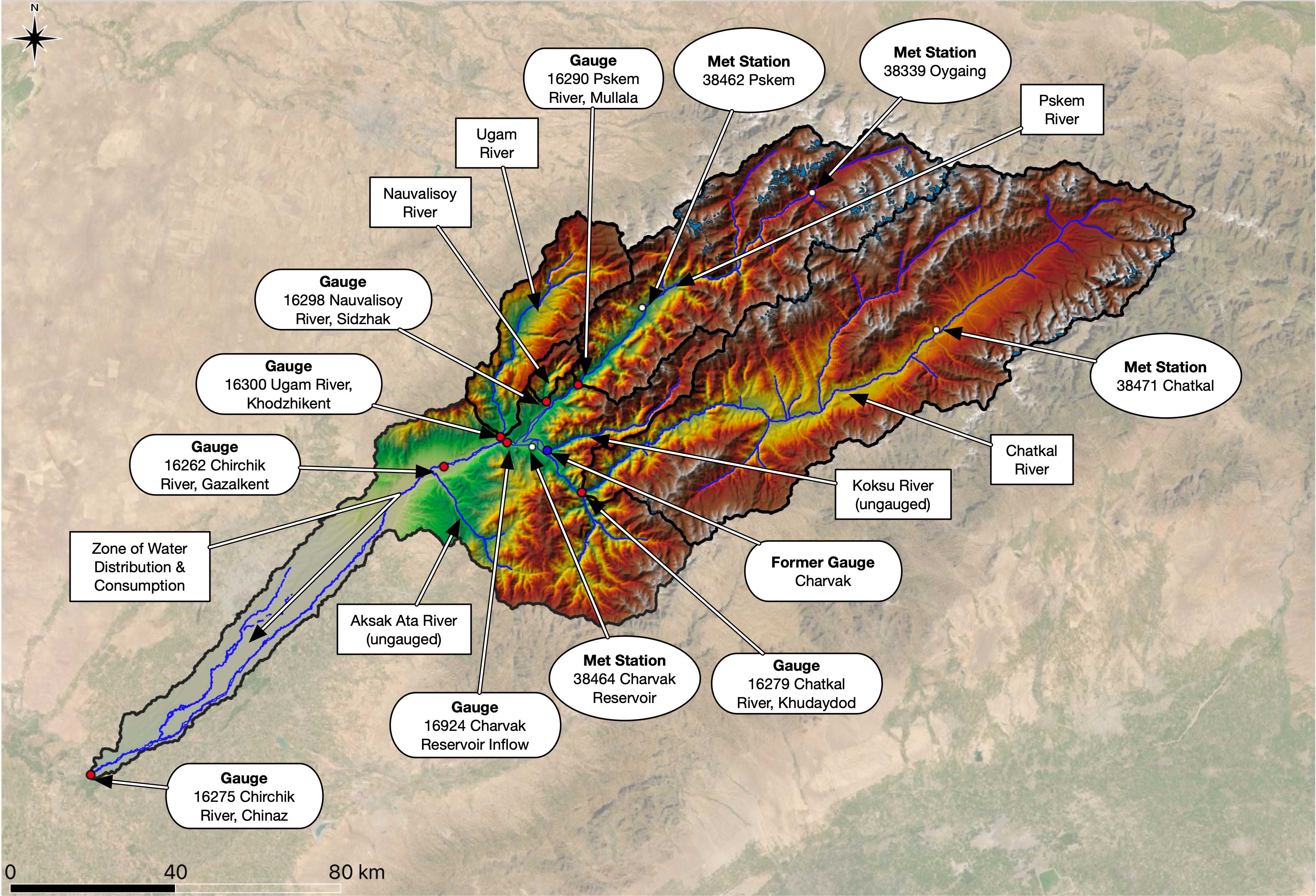
Figure 3.10: Overview over the Chirchik river basin with tributaries and the location of the main gauging stations in the zone of runoff formation and near the confluence with the Syr Darya.
Figure 3.10 shows a comprehensive overview of the Chirchik river basin and its tributaries as well as relevant modern gauging stations. Gauges are indicated with the semi-round shapes and the corresponding five digit official code as utilized by the Uzbek Hydrometeorological Service (HMS) indicated. The virtual gauge is not a real gauge in the sense that reservoir inflow is calculated from all contributing tributary flow components, i.e. Chatkal river, Pskem river, Nauvalisoy and Koksu Rivers.
Koksu however, with a basin area of 392 km\(^2\), is ungauged. Its discharge contribution is calculated using an established empirical relationship between discharge in Chatkal River and discharge in Koksu. The empirical relationship is derived further below in Section ??. First, we now turn our attention to the description of key hydrological basin features.
3.2.2 Hydrology
This Section uses a number of available data that are available to characterize the Chirchik River Basin from the hydro-climatological perspective. Data access and modeling is further described in Chapter @ref{HydroModelsEmpiricalModels} in Part II of this Book.
The available discharge data is shown in Figure 3.11. These are near complete historic records. See above Figure 3.10 for the station locations.
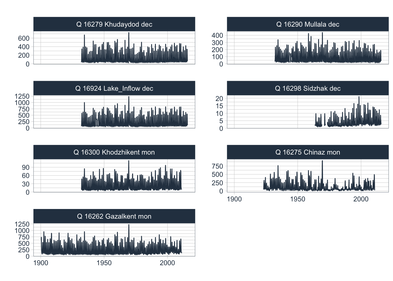
Figure 3.11: Available discharge data of Chirchik River Basin
The discharge measurements at Gazalkent gauge started already in 1900 and is one of the longest records available in Central Asia. The monthly record of the station is shown in Figure 3.12. You can zoom into the time series and investigate it in detail.
Figure 3.12: Monthly discharge at Gauge 16262, Gazalkent.
As is easily visible, the June 1969 discharge was the historic monthly mean maximum with 1’220 m3/s. The characteristics of the timeseries feature the typical snowmelt-driven runoff pattern with pronounced seasonality and interannual variability.
At Chinaz near the confluence of the Chirchik River with the Syr Darya (Gauge 16275), however, a changing discharge regime can be identified over time (Figure 3.13). The drastic decrease in discharge there is due to two effects. First, water diversions and interbasin water transfers for irrigation purposes have greatly increased over the course of the 20th century. Second, the closure of the Charvak dam in 1974 and the subsequent filling of the dam decreased discharge during the filling period. Furthermore, the interannual variability of flows decreased from there onwards due to the now regulated flow regime. This latter effect is also visible at the Gazalkent gauge. The non-stationarity in the discharge timeseries at these stations is thus explained by anthropogenic effects.
Figure 3.13: Monthly discharge at Gauge 16275, Chinaz
The effect of water diversion becomes even more apparent when the annual discharge at Gazalkent gauging station upstream of any major water diversion and at Chinaz gauge, which is in the very downstream of Chirchik River right before its confluence with the Syr Darya, are compared. The corresponding annual timeseries are shown in Figure 3.14 together with the difference of the two time series.
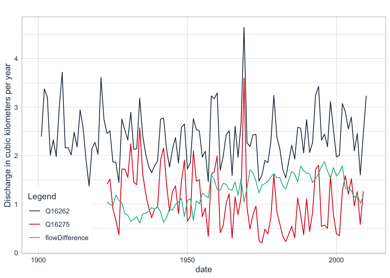
Figure 3.14: Annual discharge at Gauge 16262, Gazalkent and Gauge 16275, Chinaz and the difference of the two timeseries. The difference of the two time series is from the allocation of water for human purposes, mostly for irrigation.
Figure 3.14 shows the growing water allocation in the catchment from the 1930ies up to the end of the 20th century. Allocation grew almost 3-fold over this period. Interestingly, in the first decade of the 21st century, trends in allocation completely revered and in 2009, roughly one third of the total flow at Gazalkent was allocated consumptively. The trend reversal might be due to a change in irrigation policy, problems with intake infrastructure or both.
## # A tibble: 7 x 5
## # Groups:   code [7]
##   code   mean   min    max    sd
##   <chr> <dbl> <dbl>  <dbl> <dbl>
## 1 16262 229.   48.7 1220   186.
## 2 16275 105.    1.2  912   121
## 3 16279 116.   21.1  729   110.
## 4 16290  79.4  12.7  438    69.3
## 5 16298   3.8   0.9   21.1   2.8
## 6 16300  22.4   3.9  114    19.3
## 7 16924 205. 40.7 1231 183.| code | mean | min | max | sd |
|---|---|---|---|---|
| 16262 | 228.6 | 48.7 | 1220.0 | 186.4 |
| 16275 | 104.9 | 1.2 | 912.0 | 121.0 |
| 16279 | 115.7 | 21.1 | 729.0 | 109.9 |
| 16290 | 79.4 | 12.7 | 438.0 | 69.3 |
| 16298 | 3.8 | 0.9 | 21.1 | 2.8 |
| 16300 | 22.4 | 3.9 | 114.0 | 19.3 |
| 16924 | 205.3 | 40.7 | 1231.0 | 183.2 |
The largest left tributary to Chirchik below the Charvak reservoir Aksak Ata. The gauging station on the river got dismantled a long time ago. An average long-term mean discharge of 2.35 m\(^{3}\)/s is a solid estimated of its contribution to the overall discharge of Chirchik. Thus, if we add up long-term average discharge at Gazalkent and the one from Aksak Ata we obtain an annual norm discharge of 231 m\(^{3}\)/s.
Chirchik river is thus the biggest right-tributary to the Syr Darya. Chatkal river contributes exactly half to it (115.7 m\(^{3}\)/s) and Pskem river approximately one third (34.4% or 79.4 m\(^{3}\)/s). Nauvalisoy is only a very small river with 1.6 % runoff contribution (3.8 m\(^{3}\)/s). From the available data, the long-term average runoff contribution by the ungauged Koksu river can be estimated to be 6.4 m\(^{3}\)/s or 2.8 %. Downstream of the reservoir, Ugam river contributes an additional 9.7 % (22.4 m\(^{3}\)/s) to the total flow.
Let us now turn our attention to the seasonality of the tributaries. We exclude both, the Chinaz Gauge and Gazalkent Gauge data in our analysis for the above-mentioned reason that flow there is no longer representing a natural runoff regimes there. We thus plot seasonalities of the key gauged and unregulated tributaries , i.e. Chatkal, Pskem, Nauvalisoy and Ugam rivers in Figures ?? and ?? below.
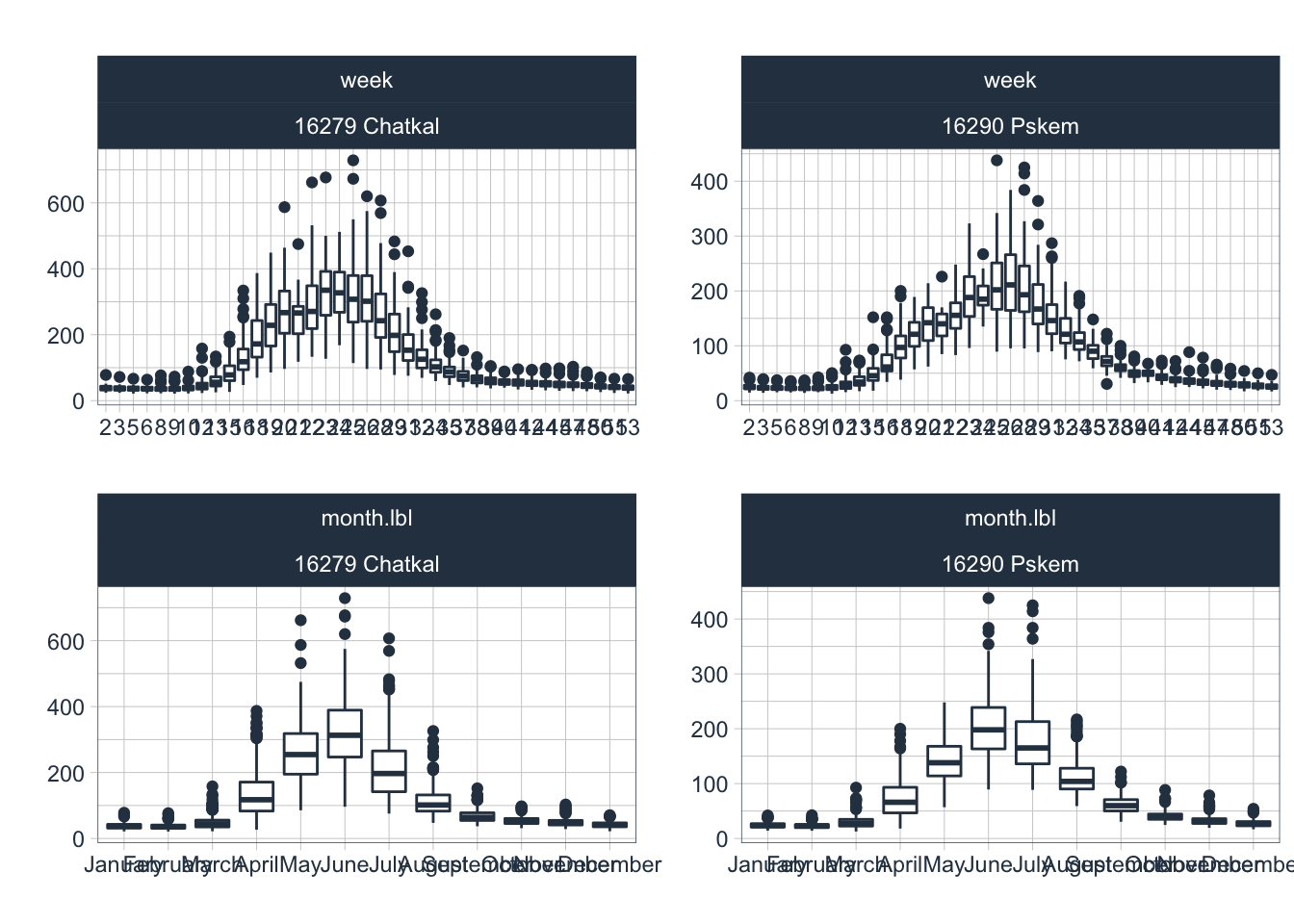
Figure 3.15: Seasonality diagnostics of the two large tributaries, i.e. the Chatkal and Pskem rivers.
Discharge seasonality of the gauging stations downstream of Charvak reservoir is shown below. Note that we only have monthly values for Ugam station which explains the appearance of the weekly plot in the upper right panel of Figure 3.16.
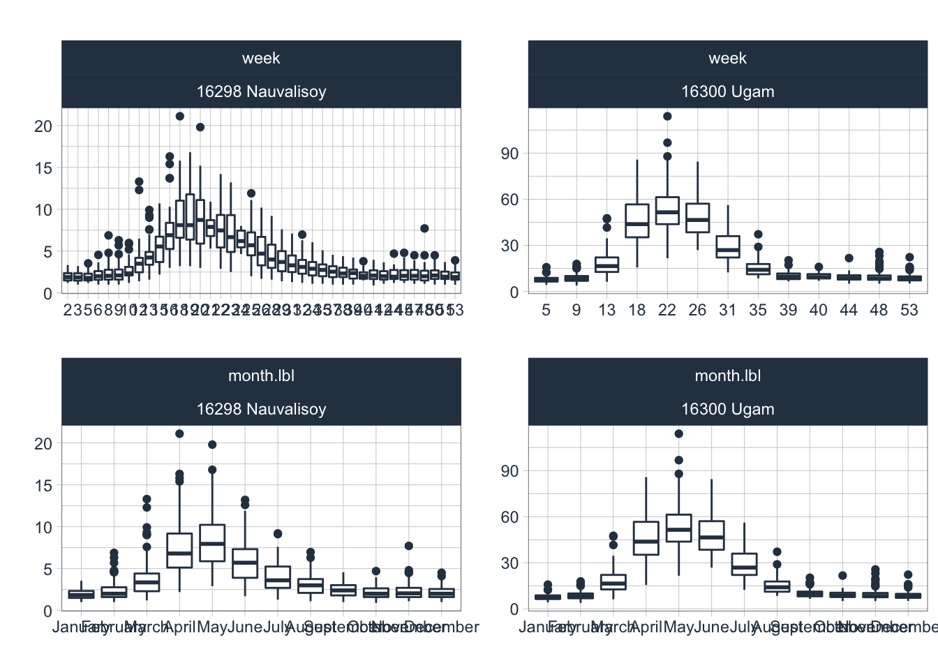
Figure 3.16: Seasonality diagnostics of the two minor tributaries taht are gauged.
The seasonality with the spring and summer runoff peaks is striking in all the rivers. Nauvalisoy discharge peaks, on average, during or around week 20. Chatkal river discharge peaks around week 23 and Pskem river around week 26. These differences can be explained with the difference in mean catchment elevations which are as follows:
- Nauvalisoy catchment: 2’160 masl,
- Ugam catchment: 803 masl,
- Chatkal catchment: 2’692 masl, and
- Pskem Catchment: 2’795 masl
where Ugam is the lowest lying and Pskem catchment the highest catchment (see also Chapter 2 for more information). Figure 3.17 shows the hypsometric curves of the main tributaries to the Chirchik River.
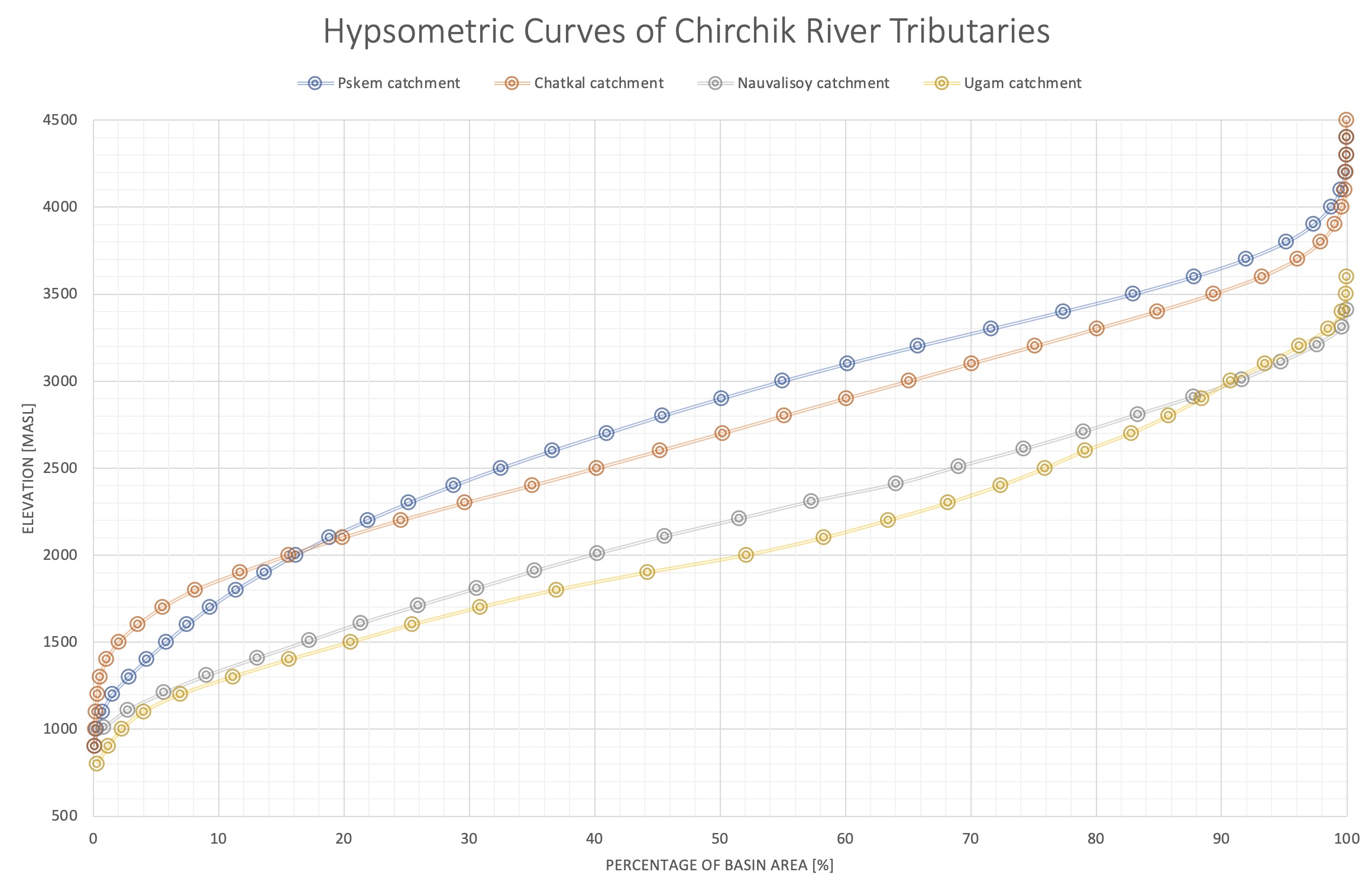
Figure 3.17: Hypsometric Curves of the tributaries to the Chirchik River Basin.
Using a LOESS smoother, we can remove discharge time series seasonality and catch a glimpse of the underlying longterm trends. This is shown for gauging station 16294, i.e. the inflow to the Charvak Reservoir, in Figure 3.18. If anything, a slightly increasing trend in mean discharge can be observed over the last 40 years. We will further discuss this finding also in the context of the analysis of the meteorological data record in the next Section.
Figure 3.18: Changes in mean monthly discharges are plotted with black lines over the entire observational record for Charvak Reservoir gauge (16924).The blue line shows a smoothed trend using a LOESS-smoother.
But what about changes for particular seasons and months? To understand these changes, we plot monthly average data grouped together individually for all months. Figure 3.19 shows the resulting graphs together with their best fit regression lines for each month. Several interesting observations can be done.
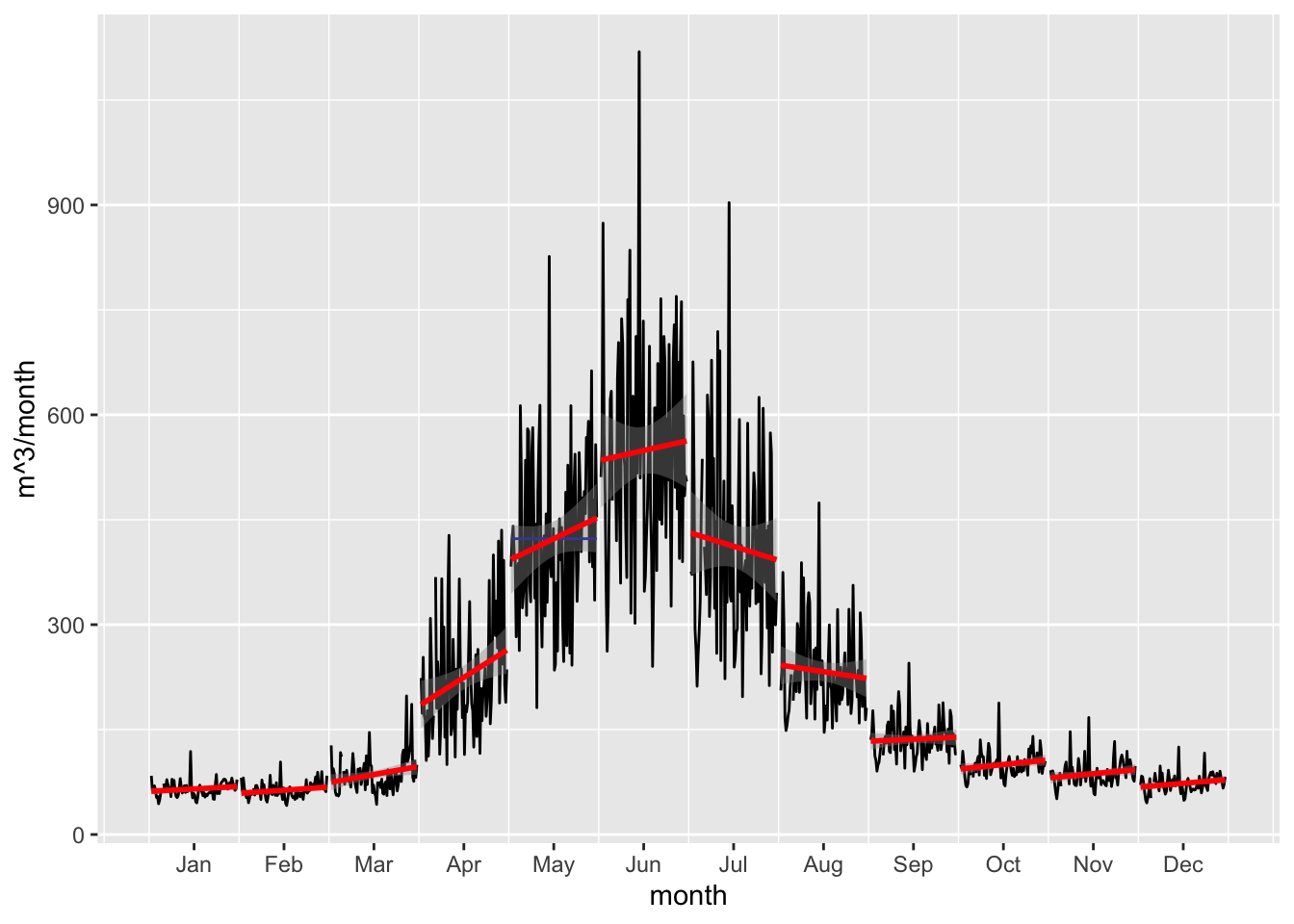
Figure 3.19: Changes in mean monthly discharges are plotted with black lines over the entire observational record for Charvak Reservoir gauge (16924).The red lines are the per month best fit regression lines.
First, cold season discharge in quarter 1 (Q1) and Q4 have a slightly increasing trend. Converse to this, the warm season quarterly trends are not uniform where Q2 trends are strongly increasing and Q3 trends are markedly decreasing. This is in line with what one would expect from a warming climate, i.e. that the snow-melt driven hydrograph peak flows shift in their timing towards earlier towards spring. At the same time, Q3 warm season discharge diminishes because of the earlier snowmelt, assuming no changes in the precipitated water. We will investigate the available climate and precipitation record in the following section.
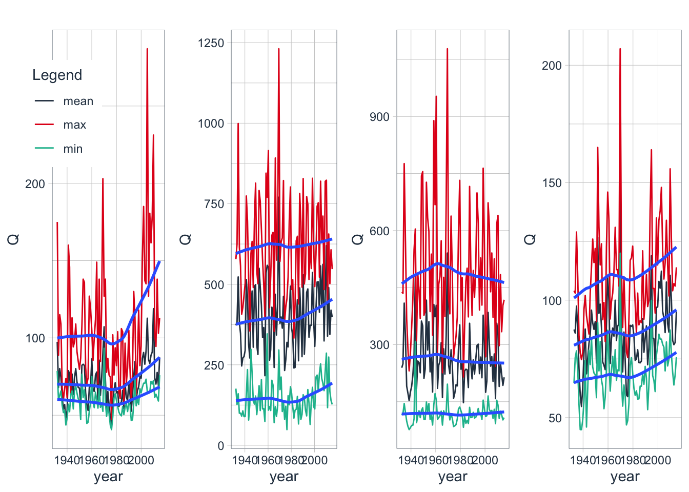
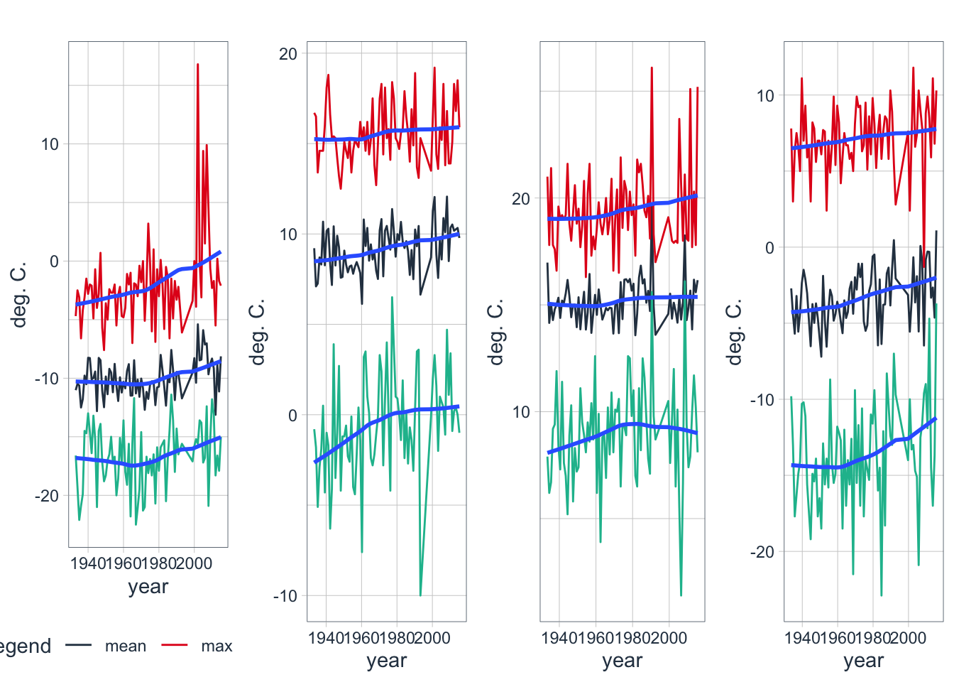
Figure 3.20: The plates show mean, minimum and maximum quarterly discharges for Q1 (upper left plate), Q2 (upper right plate), Q3 (lower left plate) and Q4 (lower right plate). All values are in mean quarterly discharge per second
The development of the quarterly minimum, maximum and mean discharge Q over the years for Gauge 16924 (Charvak reservoir inflow) is shown in Figure 3.20. The increasing trends in cold season discharge (Q1 and Q4) is confirmed. In these quarters, minimum, mean and maximum discharges appear to increase with a probably link to temperature increases during these quarters (see Section ?? for a discussion). In Q2, minimum and mean discharges have an increasing trend. In Q3, maximum discharge appears to decrease over time.
3.2.3 Climate
Long-term climate data from three different stations located in the vicinity and upstream of Charvak Reservoir is available. The stations are meteostation 38642 and 38339, both in Pskem River Basin, Meteostation 38471, Chatkal River Basin and Meteostation 38464 in the vicinity of the Charvak Reservoir (see also Figure 3.10 above for their locations.
The raw temperature data is shown in Figure 3.21 whereas the per month temperature trends are shown in Figures 3.22 and 3.23. At both stations, a significant cold season warning trend is visible.
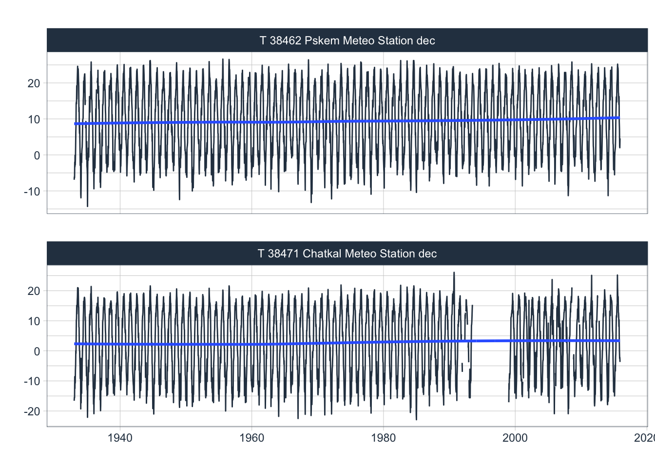
Figure 3.21: Available decadal temperature records at Pskem and Chatkal meteorological stations. The record at the Kyrgyz Chatkal Meteo Station shows a large data gap in the post-transition years. The blue trend lines (LOESS smoother) indicate an increasing temperature trend at both mountain stations.
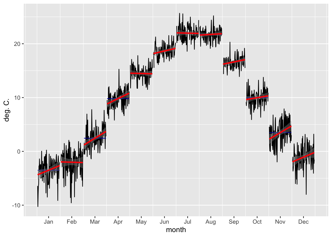
Figure 3.22: Changes in mean monthly temperatures are plotted with black lines over the entire observational record for Pskem meteorological station.The red lines are the per month best fit regression lines.
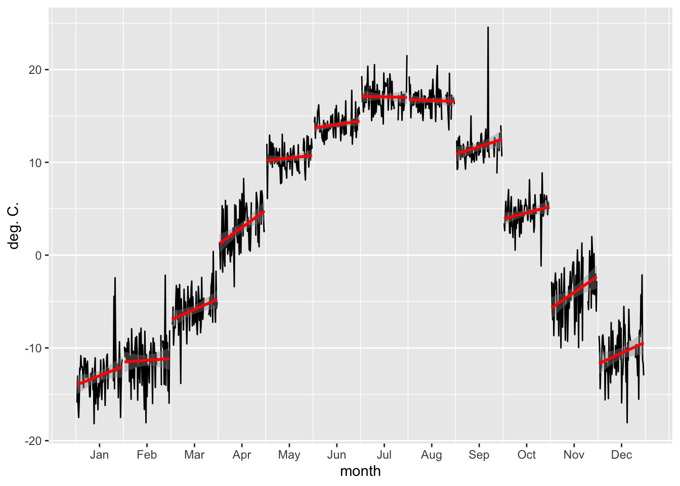
Figure 3.23: Changes in mean monthly temperatures are plotted with black lines over the entire observational record for Pskem meteorological station. The red lines are the per month best fit regression lines. The peak in the month of September is an outlier.
Similarily to the analysis carried out above for the development of quarterly flows, we can analyze the development of quarterly temperature statistics. Figure (fig:quarterlyMeanMinMaxT_38462) shows the result.
(#fig:quarterlyMeanMinMaxT_38462)Development of mean, minimum and maximum quarterly temperatures for Q1 at Station 38462
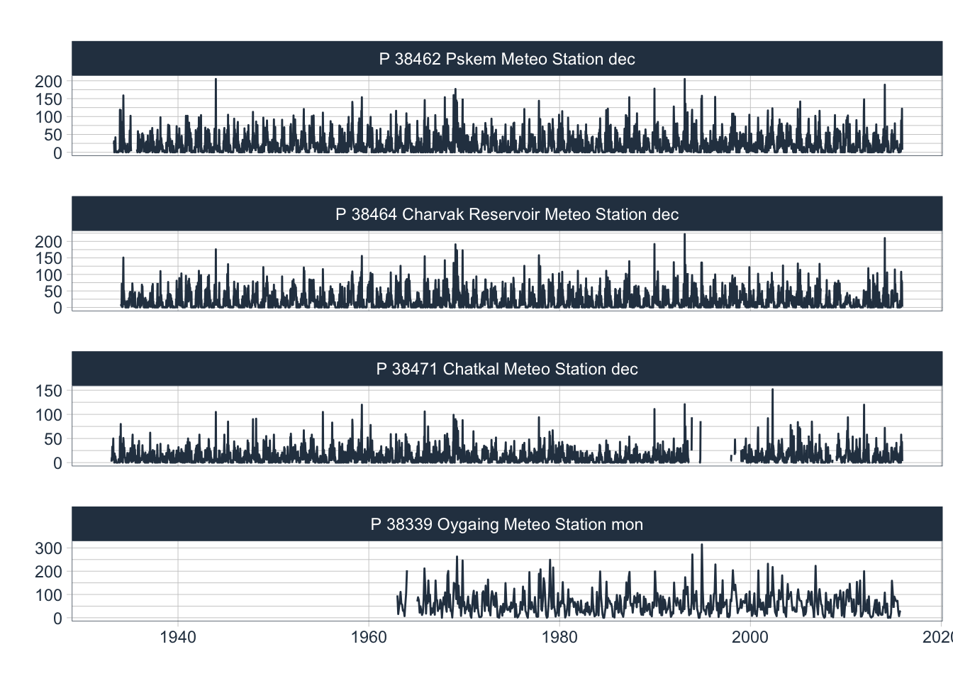
Figure 3.24: Available decadal and monthly data records from different meteorological stations that are located in the zone of runoff formation. As in the case of temperature, the precipitation record at the Kyrgyz Chatkal Meteo Station shows a large data gap in the post-transition years.
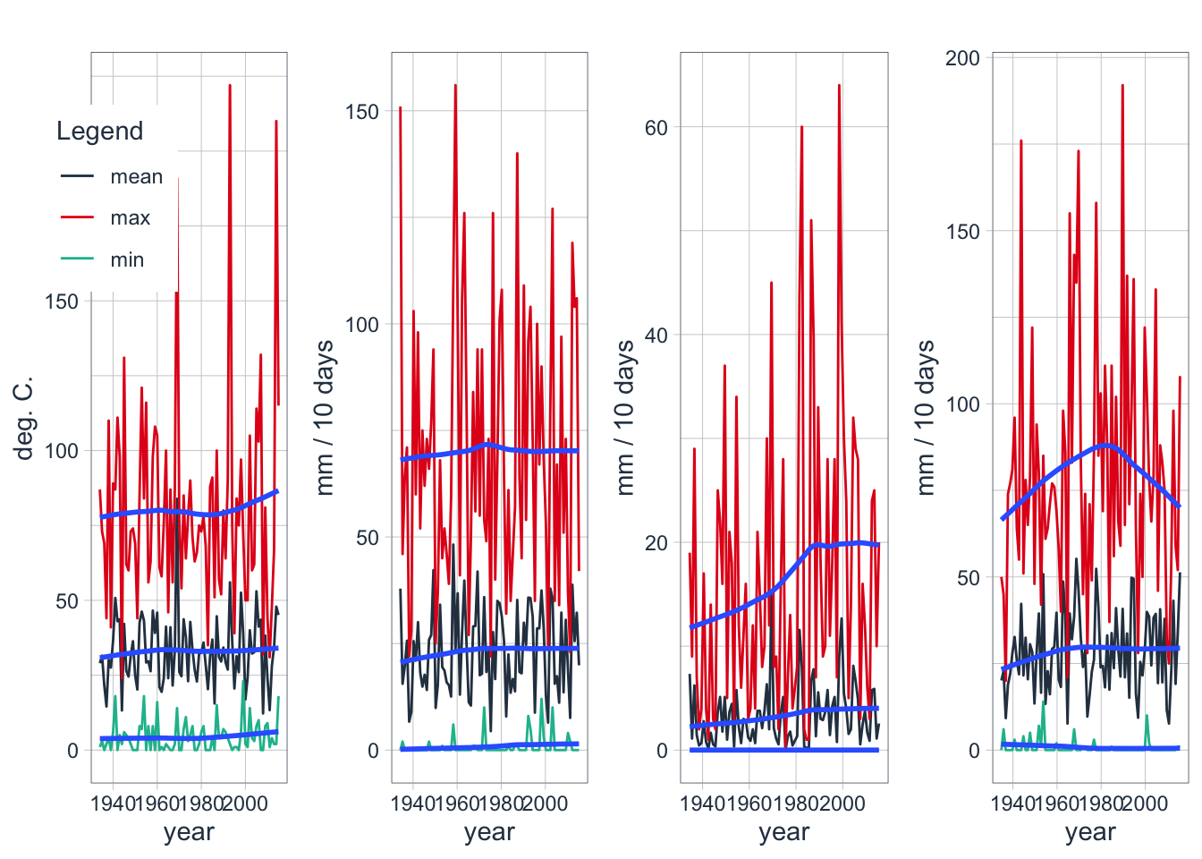
Figure 3.25: Development of mean, minimum and maximum quarterly temperatures for Q1 at Station 38462
Investigate temperature precipitation link
q1TP <- left_join(q1T ,q1P ,by=c('date','name')) %>% rename(T=value.x,P=value.y)
p1 <- q1TP %>% na.omit() %>% ggplot(aes(x=T,y=P)) + geom_point() + geom_smooth(formula = y ~ x,method = "lm")
q2TP <- left_join(q2T ,q2P ,by=c('date','name')) %>% rename(T=value.x,P=value.y)
p2 <- q2TP %>% na.omit() %>% ggplot(aes(x=T,y=P)) + geom_point() + geom_smooth(formula = y ~ x,method = "lm")
q3TP <- left_join(q3T ,q3P ,by=c('date','name')) %>% rename(T=value.x,P=value.y)
p3 <- q3TP %>% na.omit() %>% ggplot(aes(x=T,y=P)) + geom_point() + geom_smooth(formula = y ~ x,method = "lm")
q4TP <- left_join(q4T ,q4P ,by=c('date','name')) %>% rename(T=value.x,P=value.y)
p4 <- q4TP %>% na.omit() %>% ggplot(aes(x=T,y=P)) + geom_point() + geom_smooth(formula = y ~ x,method = "lm")

p <- list(p1,p4)
cowplot::plot_grid(plotlist = p,nrow = 1,ncol = 2)
Investigate temperature discharge link
q1TQ <- left_join(q1T ,q1Q ,by=c('date','name')) %>% rename(T=value.x,Q=value.y)
p1 <- q1TQ %>% na.omit() %>% ggplot(aes(x=T,y=Q)) + geom_point() + geom_smooth(formula = y ~ x,method = "lm")
q2TQ <- left_join(q2T ,q2Q ,by=c('date','name')) %>% rename(T=value.x,Q=value.y)
p2 <- q2TQ %>% na.omit() %>% ggplot(aes(x=T,y=Q)) + geom_point() + geom_smooth(formula = y ~ x,method = "lm")
q3TQ <- left_join(q3T ,q3Q ,by=c('date','name')) %>% rename(T=value.x,Q=value.y)
p3 <- q3TQ %>% na.omit() %>% ggplot(aes(x=T,y=Q)) + geom_point() + geom_smooth(formula = y ~ x,method = "lm")
q4TQ <- left_join(q4T ,q4Q ,by=c('date','name')) %>% rename(T=value.x,Q=value.y)
p4 <- q4TQ %>% na.omit() %>% ggplot(aes(x=T,y=Q)) + geom_point() + geom_smooth(formula = y ~ x,method = "lm")

p <- list(p1,p4)
cowplot::plot_grid(plotlist = p,nrow = 1,ncol = 2)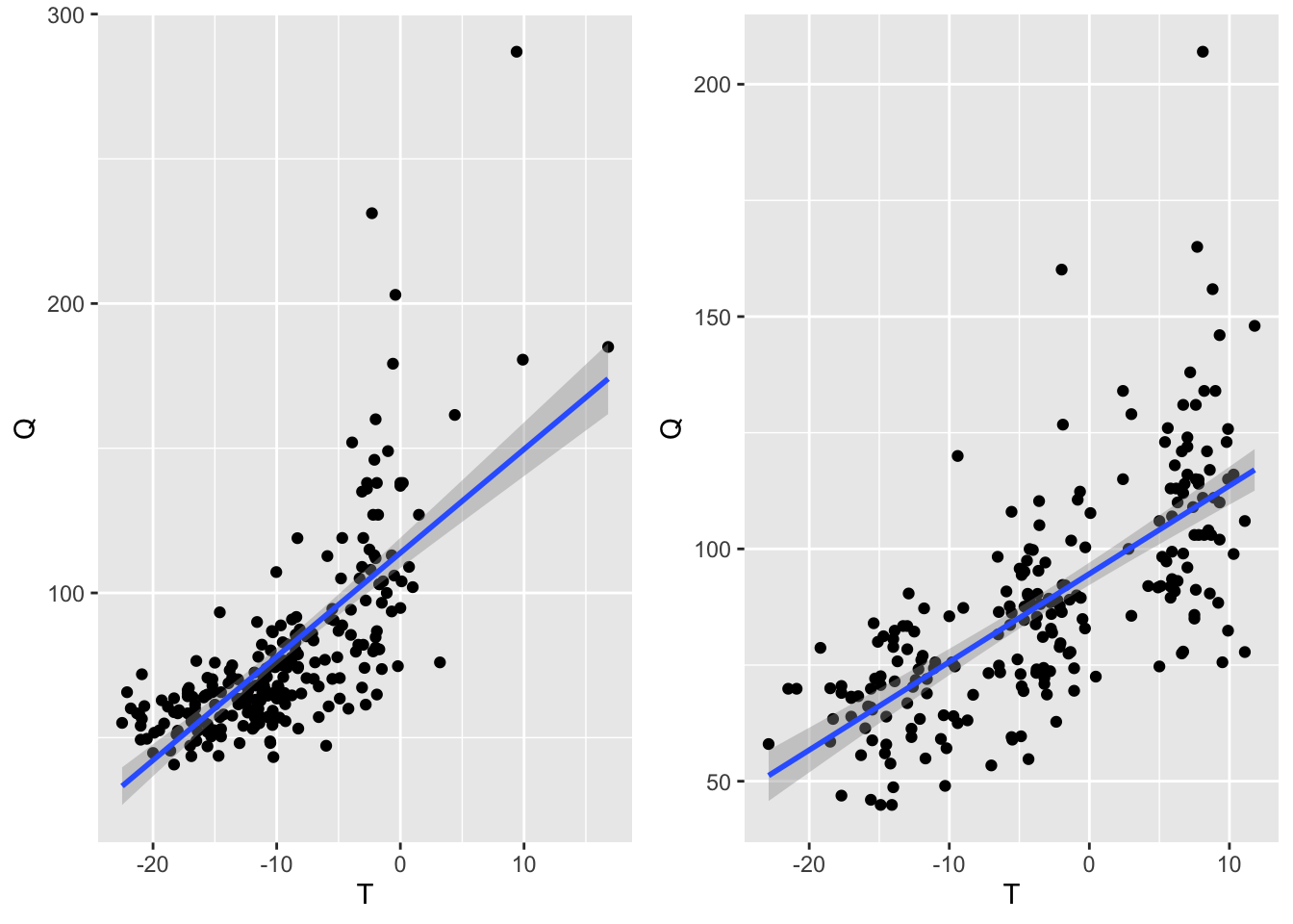
Precipitation - Discharge Link
q1PQ <- left_join(q1P,q1Q ,by=c('date','name')) %>% rename(P=value.x,Q=value.y)
p1 <- q1PQ %>% na.omit() %>% ggplot(aes(x=P,y=Q)) + geom_point() + geom_smooth(formula = y ~ x,method = "lm")
q2PQ <- left_join(q2P,q2Q ,by=c('date','name')) %>% rename(P=value.x,Q=value.y)
p2 <- q2PQ %>% na.omit() %>% ggplot(aes(x=P,y=Q)) + geom_point() + geom_smooth(formula = y ~ x,method = "lm")
q3PQ <- left_join(q3P,q3Q ,by=c('date','name')) %>% rename(P=value.x,Q=value.y)
p3 <- q3PQ %>% na.omit() %>% ggplot(aes(x=P,y=Q)) + geom_point() + geom_smooth(formula = y ~ x,method = "lm")
q4PQ <- left_join(q4P,q4Q ,by=c('date','name')) %>% rename(P=value.x,Q=value.y)
p4 <- q4PQ %>% na.omit() %>% ggplot(aes(x=P,y=Q)) + geom_point() + geom_smooth(formula = y ~ x,method = "lm")

p <- list(p1,p2,p3,p4)
cowplot::plot_grid(plotlist = p,nrow = 1,ncol = 4)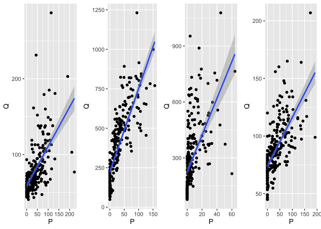
Q1 versus Q2
q1QQ <- q1Q %>% add_column(Q2=q2Q$value) %>%  rename(Q1=value)
p1 <- q1QQ %>% na.omit() %>% ggplot(aes(x=Q1,y=Q2)) + geom_point() + geom_smooth(formula = y ~ x,method = "loess")

q2QQ <- q2Q %>% add_column(Q3=q3Q$value) %>%  rename(Q2=value)
p2 <- q2QQ %>% na.omit() %>% ggplot(aes(x=Q2,y=Q3)) + geom_point() + geom_smooth(formula = y ~ x,method = "loess")

# q3QQ <- q3Q %>% add_column(Q4=q4Q$value) %>%  rename(Q3=value)
# p3 <- q3QQ %>% na.omit() %>% ggplot(aes(x=Q3,y=Q4)) + geom_point() + geom_smooth(formula = y ~ x,method = "loess")


p <- list(p1,p2)
cowplot::plot_grid(plotlist = p,nrow = 1,ncol = 2)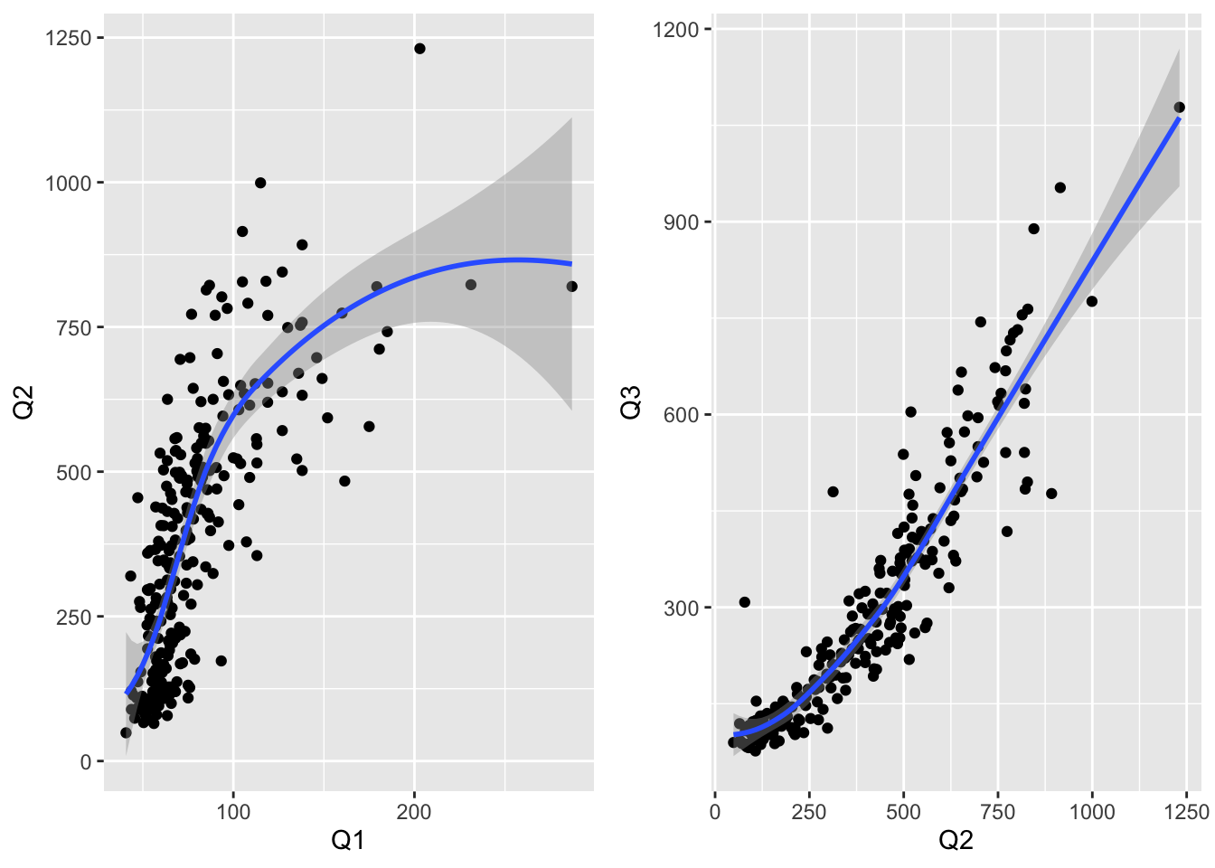
3.2.4 Discharge Estimation from the Ungauged Kosku Tributary
Before the closure of the Charvak dam and the subsequent filling of the reservoir in and after 1974, the HydroMet experts started a detailed 3-years measurement comparison campaign at Charvak gauge and at gauge 16279 in Khudaydod (see Figure 3.10). Both are located on Chatkal river. Charvak gauge had to be decommissioned after the closure of the dam because it got flooded.
The confluence of Koksu river with Charvak river is just upstream of the former Charvak gauge. Using daily data from the measurement comparisons campaign, the HydroMet experts could then relate Charvak gauge discharge to Khudaydod discharge using a linear relationship. At the same time, they were now able to relate Koksu discharge to the discharge at Chatkal River in Khudaydod in the following manner
\[ Q_{Koksu} \propto Q_{Charvak} - Q_{16279} \]
We show the procedure here. After loading the riversCentralAsia Package as shown above, the relevant daily data from 01/01/1965 - 31/12/1967 can be loaded.
KoksuDischargeDerivation <- riversCentralAsia:::KoksuDischargeDerivation # load DataPlease not that, unless otherwise mentioned, all data from discharge meteorological stations utilized in this book are from the Uzbek HMS.
The data is stored in long format, meaning that measurements in time and for the two gauging stations are just stacked on top of each other in one long table. For the purpose here, we prefer the wide format where we have one date column with unique dates and then the data listed for each station in corresponding columns.
KoksuDischarge_wide <- KoksuDischargeDerivation %>% pivot_wider(id_cols = 'date',values_from = 'data',names_from = "code")
KoksuDischarge_wide
## # A tibble: 988 x 3
## date Charvak `16279`
## <date> <dbl> <dbl>
## 1 1965-01-01 35.6 33.4
## 2 1965-01-02 35.6 32.4
## 3 1965-01-03 33 30.4
## 4 1965-01-04 33 29.4
## 5 1965-01-05 33 30.4
## 6 1965-01-06 33 30.4
## 7 1965-01-07 34.3 31.4
## 8 1965-01-08 35.6 32.4
## 9 1965-01-09 38.4 34.4
## 10 1965-01-10 35.6 32.4
## # … with 978 more rowsThe runoff contribution of Koksu can be calculated in a simple manner.
# Adding Koksu discharge to the dataframe
KoksuDischarge_wide <- KoksuDischarge_wide %>% mutate(Koksu = Charvak - `16279`)
KoksuDischarge_wide
## # A tibble: 988 x 4
## date Charvak `16279` Koksu
## <date> <dbl> <dbl> <dbl>
## 1 1965-01-01 35.6 33.4 2.20
## 2 1965-01-02 35.6 32.4 3.20
## 3 1965-01-03 33 30.4 2.6
## 4 1965-01-04 33 29.4 3.6
## 5 1965-01-05 33 30.4 2.6
## 6 1965-01-06 33 30.4 2.6
## 7 1965-01-07 34.3 31.4 2.9
## 8 1965-01-08 35.6 32.4 3.20
## 9 1965-01-09 38.4 34.4 4
## 10 1965-01-10 35.6 32.4 3.20
## # … with 978 more rowsThe relationship can now be visualized.
# and visualize
ggplot(KoksuDischarge_wide, aes(`16279`, Koksu)) +
  geom_point() +
  xlab(bquote('Discharge at Gauge 16279 Khudaydod in'~m^3/s)) +
  ylab (bquote('Koksu river discharge in'~m^3/s))
We can perform a linear regression to related discharge at Khudaydod to the one at Koksu. The coefficients of the linear regression can be obtained in the following way:
lm <- lm(Koksu ~ 0 + `16279`,KoksuDischarge_wide)
summary(lm)
##
## Call:
## lm(formula = Koksu ~ 0 + `16279`, data = KoksuDischarge_wide)
##
## Residuals:
## Min 1Q Median 3Q Max
## -38.295 -5.867 -1.918 1.416 120.419
##
## Coefficients:
## Estimate Std. Error t value Pr(>|t|)
## `16279` 0.14469 0.00298 48.55 <2e-16 ***
## ---
## Signif. codes: 0 '***' 0.001 '**' 0.01 '*' 0.05 '.' 0.1 ' ' 1
##
## Residual standard error: 12.4 on 987 degrees of freedom
## Multiple R-squared: 0.7049, Adjusted R-squared: 0.7046
## F-statistic: 2357 on 1 and 987 DF, p-value: < 2.2e-16Please note, in the specification of the linear model we add the 0 term to force the regression through the origin. Hence, the discharge of Koksu River can be estimated to be
\[ Q_{Koksu} = 0.145 * Q_{Khudaydod} \]