5.4 Data on Climate Projections
In order to look into the future with a hydrological model for exploring climate scenarios, it needs to be fed with those scenarios. The production of these scenarios in a way resembles the steps described for the reanalysis data but also differs in some marked way. Let us outline them first before diving into the details.
First, a baseline period is defined which serves as a reference against which future climate impacts are assessed. Second, the future period of interest for the investigation of climate impacts needs to be defined and climate scenarios identified that cover the area and period of interest. The future climate scenarios are outputs from global climate models (GCMs). These GCMs normally generate monthly data as a function of representative concentration pathways (called RCPs). They describe possible futures as a function of different atmospheric CO2-concentration scenarios.
We focus the discussion here on the RCP 4.5 and RCP 8.5 concentration scenarios. According to the IPCC, RCP 4.5 is an intermediate scenario where CO2 emissions peak around 2040, then decline. Compared to this, RCP 8.5 is generally considered to be a worst case climate change scenario. Very detailed information regarding these scenarios, their underlying assumptions and assumptions can be found on the dedicated website served by the Intergovernmental Panel for Climate Change (IPCC). See the link here.
![The development of greenhouse gas concentrations during the 21st century as a function of the corresponding scenario. We focus here on RCP4.5 and RCP8.5. Source: [@van_Vuuren_2011]](_bookdown_files/FIG_DATA/greenhouseGasConcetrations_RCP.jpg)
Figure 5.37: The development of greenhouse gas concentrations during the 21st century as a function of the corresponding scenario. We focus here on RCP4.5 and RCP8.5. Source: (Vuuren et al. 2011)
5.4.1 High Res. Monthly Climate Time Series for 2006 - 2100
The recently released high-resolution climate scenario datasets described by (Karger et al. 2020) are utilized here to study climate impacts in river basins in the Central Asia region. The authors of the aforementioned paper present GCM output for monthly precipitation, mean minimum as well as maximum monthly temperatures that has been downscaled using the CHELSA algorithm.11 The data can be found here https://www.envidat.ch/#/metadata/chelsa_cmip5_ts.
We download data from 3 out of the 4 available downscaled GCM runs for further analysis and processing. These are outputs from the Coupled Model Intercomparison Project phase 5 (CMIP5) and are gridded monthly time series from the years 2006 through 2100 with a spatial resolution of 0.049 degrees (see again (Karger et al. 2020) for all the details). The three models from which data were taken are: CMCC-CM run by the Centro Euro-Mediterraneo per I Cambiamenti Climatici (CMCC); MIROC5 run by the University of Tokyo; and ACCESS1-3 run by the Commonwealth Scientific and Industrial Research Organization (CSIRO) and Bureau of Meteorology (BOM), Australia (Karger et al. 2020).
First, the data is downloaded and stored locally for RCP 4.5 and RCP 8.5. Then, as in the case of the original CHELSA data (see Section 5.3.2.3, the monthly gridded precipitation time series are bias corrected using the monthly correction factors as report by (Beck et al. 2020d) and finally, mean monthly temperature fields are generated from the minimum and maximum monthly temperatures. The resulting data available for the Central Asia domain are available for download via this link12.
As in the case of the ERA5 data, these GCM data need to be made available for all the elevation bands. By providing a proper shapefile that contains sub-basin specific elevation bands of a catchment, the function riversCentralAsia::downscale_ClimPred_monthly_BasinElBands() can be used to compute these data. The function processes the climate projection raster bricks with precipitation_flux and air_temperature (tasmin, tasmean and tasmax) and computes elevation band statistics. The next code block provides sample code on how to use riversCentralAsia::downscale_ClimPred_monthly_BasinElBands().
Please be aware that if you want to try this locally on your computer, it is required that you download the entire high resolution climate scenarios for the Central Asia on your local machine. The data are available under this link. The whole process is shown here using a shapefile of the Gunt river basin that explicitly includes Lake Yashikul in the upstream of the basin. In lieu of this example, your own catchment subbasin file can easily be loaded and provided.
# Data
climScen_Path <- '../HydrologicalModeling_CentralAsia_Data/CentralAsiaDomain/PROJECTIONS/' # This Path would need to be adjusted for in case the directory with the climate projections is stored elsewhere.
rcp <- c('rcp45','rcp85')
cModelList <- c('ACCESS1-3','CMCC-CM','MIROC5')
# Catchment Shapefile
elBands_shp <- st_read('./data/AmuDarya/GuntYashikul/GeospatialData/subbasins_Z.shp')
# Ensure Projection is latlon
elBands_shp_latlon <- sf::st_transform(elBands_shp,crs = sf::st_crs(4326))
# Unused catchments in RSMinerve? Preprocess Shapefile: This is specific for the Gunt-Yashikul model and can be removed if not required or change accordingly.
elBands_shp_latlon <- elBands_shp_latlon %>% dplyr::slice(-1:-3)

# Fancy trick to generate an empty dataframe with column names from a vector of characters.
namesElBands <- elBands_shp_latlon$name
dataElBands_df <- namesElBands %>% purrr::map_dfc(setNames, object = base::list(base::logical()))

# Start and end years of climate projections
startY <- 2006
endY <- 2100

# Search pattern for file list
fileListSearchPattern <- "2006-2100"

# Generate downscaled climate scenario files and store files in corresponding directory
# RCP45
pathN <- paste0(climScen_Path,'rcp45','/','ACCESS1-3','/')
downscaled_ClimPred_rcp45_ACCESS1_3 <-downscale_ClimPred_monthly_BasinElBands(pathN,fileListSearchPattern,
                                                                              startY,endY,elBands_shp_latlon)

pathN <- paste0(climScen_Path,'rcp45','/','CMCC-CM','/')
downscaled_ClimPred_rcp45_CMCC_CM <- downscale_ClimPred_monthly_BasinElBands(pathN,fileListSearchPattern,
                                                                              startY,endY,elBands_shp_latlon)
pathN <- paste0(climScen_Path,'rcp45','/','MIROC5','/')
downscaled_ClimPred_rcp45_MIROC5 <- downscale_ClimPred_monthly_BasinElBands(pathN,fileListSearchPattern,
                                                                              startY,endY,elBands_shp_latlon)

# RCP85
pathN <- paste0(climScen_Path,'rcp85','/','ACCESS1-3','/')
downscaled_ClimPred_rcp85_ACCESS1_3 <-downscale_ClimPred_monthly_BasinElBands(pathN,fileListSearchPattern,
                                                                              startY,endY,elBands_shp_latlon)
pathN <- paste0(climScen_Path,'rcp85','/','CMCC-CM','/')
downscaled_ClimPred_rcp85_CMCC_CM <- downscale_ClimPred_monthly_BasinElBands(pathN,fileListSearchPattern,
                                                                              startY,endY,elBands_shp_latlon)
pathN <- paste0(climScen_Path,'rcp85','/','MIROC5','/')
downscaled_ClimPred_rcp85_MIROC5 <- downscale_ClimPred_monthly_BasinElBands(pathN,fileListSearchPattern,
                                                                              startY,endY,elBands_shp_latlon)

# Store files if required in the corresponding catchment-specific folder. For the example presented here, this is in the following directory.
# basin_climScen_Path <- './data/AmuDarya/GuntYashikul/ClimateProjections/'
#
# climScen_fileList <- c('downscaled_ClimPred_rcp45_ACCESS1_3', 'downscaled_ClimPred_rcp45_CMCC_CM',
#                'downscaled_ClimPred_rcp45_MIROC5','downscaled_ClimPred_rcp85_ACCESS1_3',
#                'downscaled_ClimPred_rcp85_CMCC_CM','downscaled_ClimPred_rcp85_MIROC5')
#
# save(climScen_fileList,list = climScen_fileList,file = paste0(basin_climScen_Path,'climScen_monthly','.rda'))
It is important to mention that precipitation is stored in units of kg/m2/s in these climate projection data. How do we arrive at mm/month in order to make these data compatible with the ERA5 data? To answer this question, let us make a little thought experiment. What happens when you pour 1 kg of water on a 1 m2 big patch? 1 kg corresponds to 1 liter that corresponds to 10-3 m3. So, very simply, this amount of water poured on such a patch generates a water height of exactly 1 mm. Using this equivalence, we can rewrite the unit kg/m2/s to mm/s. Finally, in order to arrive at mm/day, for example, we just multiply the data by 60x60x24 = 86’400 which are the number of seconds in a day. Since the climate model output is in monthly time intervals, we need mm/month and hence would also need to multiply by the number of days in the corresponding month.
As discussed, these GCM data are high spatial resolution monthly future climate fields which we downscaled on the corresponding catchment shapefile with its subbasins and elevation bands. All good. But how do we arrive at climate fields that also have a high temporal resolution (hourly time resolution in this case) so that we can drive the RS MINERVE hydrological model with the required input data? The solution is shown in the following Section @ref(Data::WeatherGenerator) using a weather generator. A weather generator is a stochastic model that produces daily weather variables which can then be converted to hourly fields.
5.4.2 Using a Weather Generator to Simulate Daily Future Climate
5.4.2.1 Background and Input File Generation
Stochastic weather generators are probabilistic models that are used to simulate weather data at a specific site or region by analyzing historical weather data and then generating a time-series of weather variables with statistical properties identical to the historical data (Birt et al. 2010). We demonstrate the use of RMAWGEN, a stochastic weather generator available for the R environment. Further information on RMAWGEN can be found here https://github.com/ecor/RMAWGEN and under the links provided via the package information on GitHub.
While the weather generator is relatively poorly documented, a useful albeit very technical presentation of the tool is available here. Furthermore, the functions are documented well in the latest development version of the package. The package can be installed in the following way directly from GitHub:
# Install GitHub version
library(devtools)
install_github("ecor/RMAWGEN")
library(RMAWGEN)
RMAWGEN allows for the generation of daily temperature and precipitation scenarios that are conditioned on monthly climate scenario totals as given by the GCM model outputs. This is the key idea. Using again an example of the Gunt-Yashikul river basin, the following code block shows how to use the function prepare_RMAWGEN_input_data() for the preparation of the relevant RMAWGEN input data files so that the weather generator can be run.
# Load and process RS MINERVE csv database file
filePath <- './data/AmuDarya/GuntYashikul/RSMinerve/'
fileName <- 'Gunt_Yashikul_1981_2013_db.csv'
era5_gunt_yashikul_1 <- read.table(paste0(filePath,fileName),sep=',') %>% as_tibble()

# Deleting unused catchments in the tibble. These catchments are not modeled later in RS MINERVE, so we can safely delete them here. Note that this operation is specific to the Gunt-Yashikul model and does not generalize to other catchments.
idx2del <-
  (era5_gunt_yashikul[1,]=='Gunt_DS_1')|
  (era5_gunt_yashikul[1,]=='Gunt_DS_2')|
  (era5_gunt_yashikul[1,]=='Gunt_DS_3')
era5_gunt_yashikul <- era5_gunt_yashikul %>% dplyr::select(which(!idx2del))

# Generate the input files for the stochastic weather generator.
station_data <- prepare_RMAWGEN_input_data(era5_gunt_yashikul)
# In case variables in station_data list should not be made available directly on the workspace, on can comment out the following line of code.
station_data %>% list2env(.,envir = .GlobalEnv) # Send list variables to global environment.
The function returns a list rmawgen_input_files with all key information that can be unlisted using rmawgen_input_files %>% list2env(.,envir = .GlobalEnv). Data returned are:
STATION_NAMES: Character vector of station names (effectively, these are just the subbasin names extracted from the RS MINERVE input file).
ELEVATION: Mean elevation of the stations
STATION_LATLON: Matrix with station names, latitude and longitude
LOCATION: Same as the station name, used above.
PRECIPITATION: Tibble containing daily precipitation for each station
TEMPERATURE_MIN: Minimum daily temperature (calculated from the ERA5 hourly data stored in the RS MINERVE csv file)
TEMPERATURE_MAX: Maximum daily temperature (ditto)
A weather generator is a type of model that uses input data to simulate output variables, i.e. daily precipitation and minimum as well as maximum temperatures. Exactly like for example a hydrological runoff model, the stochastic weather generator model depends on input parameters. Different input parameter configuration lead to different model performance / outcomes. How are these parameters calibrated and how is such a model validated when we do not have calibration and validation sets available for the future periods for which climate impacts need to be studied?
The way to do this is to calibrate and validate the stochastic weather generator with reanalysis ERA5 data for each elevation band in the catchment of interest. In other words, we assume that each elevation band contains a representative meteorological station for which we have the ERA5 data available which is used to calibrate and validate daily weather generator models. In this context, the terms elevation bands and meteorological stations are used interchangeably.
The key question to be answered then is whether or not the model is able to reproduce the statistical characteristics of the ERA5 dataset for each elevation band/station. If yes, we can safely assume that the weather generator can in a more or less realistic manner generate stochastic future daily climate fields that are conditioned on local conditions and on the monthly minimum and maximum temperature and precipitation fields from the climate projections.
A typical parameter set of RMAWGEN for testing different models with different parameters can be specified in the following way.
# Housekeeping
set.seed(123456) # Random generator seed is set to make results reproducible.

# Monthly climate is calculated if it is set to NULL.
PREC_CLIMATE <- NULL

# Calibration Period
year_min <- 1981
year_max <- 2013
origin <- "1981-1-1" # This is the starting date for which we have data available.

# n GPCA iterations for variable and VAR residuals
n_GPCA_iter <- 5
n_GPCA_iteration_residuals <- 5

# Autoregression orders (p) and exogenous vars
p_test <- 1
p_prec <- 3
exogen <- NULL
exogen_sim <- exogen

# number of weather realizations
nscenario <- 1

# Simulation period
year_min_sim <-  year_min # we are not yet simulating future climate but use the available data for model assessment, hence year_min_sim = year_min
year_max_sim <-  year_max # we are not yet simulating future climate but use the available data for model assessment, hence year_max_sim = year_max

# Minimum Precipitation value below which no precip is considered
valmin <- 1.0
The different parameter configurations will be used to run different stochastic weather generator models. In a validation step, the best model will be chosen as explained in the next Section 5.4.2.2.
5.4.2.2 Model Calibration & Validation for Model Selection
Different parameter combinations can be tested be setting up different models. The performance of the individual models is then assessed as a function of these configurations. We show the process by specifying 4 weather generator models, i.e. model1 through model4 and then generate the model output which is finally compared with the observed ERA5 data over the 1981 - 2013 period. The model that reproduces the observed ERA5 data in the best possible manner is then selected as the final weather generator model. The process is demonstrated here for the Gunt-Yahsikul river basin13.
# P03GPCA_prec
model1 <- ComprehensivePrecipitationGenerator(
  station = STATION_NAMES,
  prec_all = PRECIPITATION,
  year_min = year_min,
  year_max = year_max,
  p = p_prec,
  n_GPCA_iteration = n_GPCA_iter,
  n_GPCA_iteration_residuals = n_GPCA_iteration_residuals,
  exogen = exogen,
  exogen_sim = exogen_sim,
  sample = "monthly",
  mean_climate_prec = PREC_CLIMATE,
  no_spline = FALSE,
  year_max_sim = year_max_sim,
  year_min_sim = year_min_sim
  )

# P01GPCA
model2 <- ComprehensivePrecipitationGenerator(
  station = STATION_NAMES,
  prec_all = PRECIPITATION,
  year_min = year_min,
  year_max = year_max,
  p = p_test,
  n_GPCA_iteration = n_GPCA_iter,
  n_GPCA_iteration_residuals = n_GPCA_iteration_residuals,
  exogen = exogen,
  exogen_sim = exogen_sim,
  sample = "monthly",
  mean_climate_prec = PREC_CLIMATE,
  no_spline = FALSE,
  year_max_sim = year_max_sim,
  year_min_sim = year_min_sim
  )

# P03
model3 <- ComprehensivePrecipitationGenerator(
  station = STATION_NAMES,
  prec_all = PRECIPITATION,
  year_min = year_min,
  year_max = year_max,
  p = p_prec,
  n_GPCA_iteration = 0,
  n_GPCA_iteration_residuals = 0,
  exogen = exogen,
  exogen_sim = exogen_sim,
  sample = "monthly",
  mean_climate_prec = PREC_CLIMATE,
  no_spline = FALSE,
  year_max_sim = year_max_sim,
  year_min_sim = year_min_sim
  )

# P01
model4 <- ComprehensivePrecipitationGenerator(
  station = STATION_NAMES,
  prec_all = PRECIPITATION,
  year_min = year_min,
  year_max = year_max,
  p = p_test,
  n_GPCA_iteration = 0,
  n_GPCA_iteration_residuals = 0,
  exogen = exogen,
  exogen_sim = exogen_sim,
  sample = "monthly",
  mean_climate_prec = PREC_CLIMATE,
  no_spline = FALSE,
  year_max_sim = year_max_sim,
  year_min_sim = year_min_sim
  )
The performance of the 4 models can be assessed with statistical tests and graphically, with qq-plots and through the comparison of simulated versus observed monthly precipitation totals. Results are shown in the Figures below.
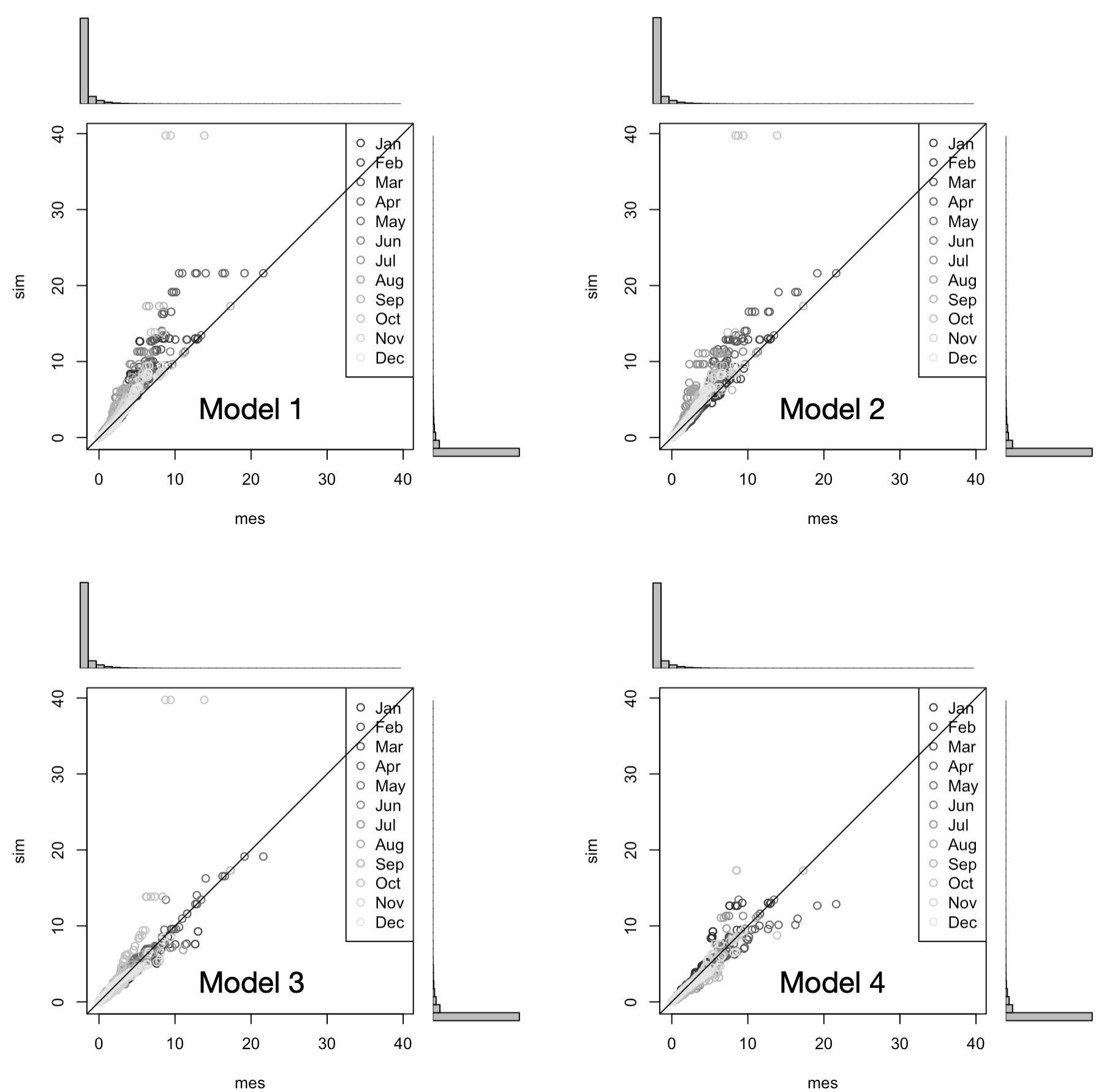
Figure 5.38: The comparison of the 4 stochastic weather generator models in terms of their abilities to reproduce monthly precipitation totals is shown for one station (elevation band Alishur_2) in the Gunt river basin. Measured monthly totals (mes) are shown on the x-axis and simulated monthly totals (sim) on the y-axis. Results indicate that precipitation totals from the models 1 and 2 are overestimated. In comparison, results from the models 3 and 4 are more balanced and not biased.
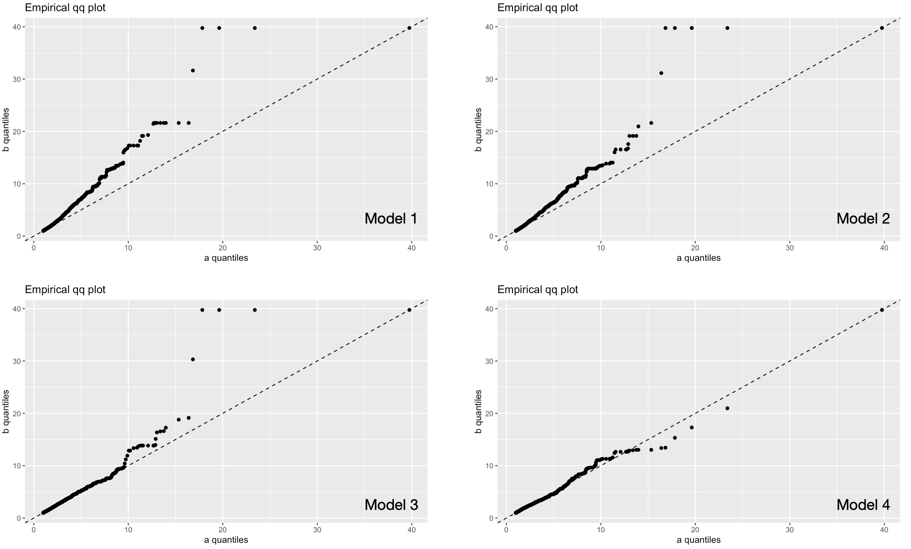
Figure 5.39: QQ-Plots of the four model results. If data plots along the diagonal line, it is an indication that the probability distribution of the simluated precipptation (y-axis) is the same as the probability distribution of the observed ERA5 precipitation (x-axis). QQ-plots of models 1 and 2 show a heavy bias whereas model 4 shows an overal satisfactory fit and thus performance.
All four models pass the multivariate Portmanteau and Breusch-Godfrey (Lagrange Multiplier) tests, which verify the absence of time-autocorrelation of the VAR(p) residuals in the modeled precipitation time series (seriality test). Furthermore, all models pass the Jarque-Bera multivariate skewness and kurtosis test, which validate the multivariate Gaussian probability distribution of the VAR(p) residuals (normality test). See (Pfaff 2008) for more information.
Figure 5.38 and Figure 5.39 show that the Model 4 provides an overall well-balanced performance. We will thus us this models to generate the future climate fields in the Gunt river basin.
Temperature is not independent of precipitation and vice versa. The two climate state variables and their changes are interlinked. In the warm season over continents, higher temperatures accompany lower precipitation amounts and vice versa. Hence, over land, strong negative correlations dominate, as dry conditions favor more sunshine and less evaporative cooling, while wet summers are cool (see e.g. IPCC Fourth Assessment Report: Climate Change 2007, Working Group I, The Physical Science Basis, Section 3.3.5, available here). Simply put, on rainy cloudy days, there is less radiation for warming the earth surface and vice versa.
This coupling needs to be taken into account when simulating weather. Therefore, we use the model4 configuration to first generate multi-site synthetic future precipitation time series. Second, we use precipitation as exogenous predictors in the temperature generation step (tasmin and tasmax). Like this, we can coupled temperature simulation to precipitation. If the results are satisfactory, we proceed with this stochastic weather model to produce future simulated weather runs that are conditioned on GCM output for the mid-21st (Period 1) and end of 21st century (Period 2).
5.4.2.3 Coupling Precipitation Realizations with Temperature
For initiating and running the weather generator, the riversCentralAsia::wgen_daily_PT() function can be used. It is a wrapper function that minimizes code reuse and allows to easily run RMAWGEN for the baseline period and/or for the future target period of the climate scenario under consideration. The use of the function is demonstrated below for a subset of 2 out of the complete set of all 17 stations in the Gunt-Yashikul catchment.
# 1. Station Data
## Load and process RS MINERVE csv database file
filePath <- './data/AmuDarya/GuntYashikul/RSMinerve/'
fileName <- 'Gunt_Yashikul_1981_2013_db.csv'
era5_gunt_yashikul <- read.table(paste0(filePath,fileName),sep=',') %>% as_tibble()

## Delete unused catchments in the Gunt-Yashikul hydrological model (this is specific to the model and does not need to be carried out normally)
idx2del <- (era5_gunt_yashikul[1,]=='Gunt_DS_1') | (era5_gunt_yashikul[1,]=='Gunt_DS_2') |
  (era5_gunt_yashikul[1,]=='Gunt_DS_3')
era5_gunt_yashikul <- era5_gunt_yashikul %>% dplyr::select(which(!idx2del))

## Generate list containing all station data (this is an input to the wgen_daily_PT() function)
station_data <- prepare_RMAWGEN_input_data(era5_gunt_yashikul)

# 2. RMAWGEN PARAMETERS
## Note: all parameteres are stored in the param list
param <- list()
## Random generator seed
param$seed <- 123456
## Monthly climate is calculated if it is set to NULL
param$PREC_CLIMATE <- NULL
## Calibration Period
param$year_min <- 1981
param$year_max <- 2013
param$origin <- "1981-1-1"
## n GPCA iterations for variable and VAR residuals
param$n_GPCA_iter <- 0
param$n_GPCA_iteration_residuals <- 0
param$n_GPCA_iter_prec <- 0
param$n_GPCA_iteration_residuals_prec <- 0
## Autoregressive order (p)
param$p <- 1
# number of weather realizations
param$nscenario <- 1
# Multi-site stations
param$station <- station_data$STATION_NAMES
# Minimum precipitation cutoff value, i.e. threshold value below which a no precipitation event is recorded [in mm/day]
param$valmin <- 1.0

# 3. Compute stochastic weather for a subset of 2 sample stations for the calibration period 1981 - 2013
clim_scen <- NULL # We not yet simulate future climate. This follows in the next Subsection below.
station_subset <- station_data$STATION_NAMES[1:2] # Selecting 2 example stations, i.e. Alishur_2 and Alishur_3. Normally, one wants to run the function for all stations.

# Return VAR model? If we set this parameter to false, the output size of the PT_sim variable will be greatly reduced.
param$returnVARModel = FALSE
# Fire up the stochastic VAR machine
PT_sim <- wgen_daily_PT(param,station_data,station_subset,clim_scen,param$returnVARModel)
The output of RMAWGEN::ComprehensivePrecipitationGenerator() and RMAWGEN::ComprehensivePrecipitationGenerator() are stored in the PT_sim list. Summary statistics of the resulting simulated climate can be obtained by using the riversCentralAsia::wgen_daily_summaryStats() function. For this, the period of interest for comparison (we call this baseline period) needs to be specified by setting param$year_min_Baseline and param$year_max_Baseline as shown below. For each station in the station subset, summary statistics can be shown.
param$year_min_Baseline <- 2004
param$year_max_Baseline <- 2013

clim_scen <- NULL

# Computing the baseline statistics and comparing it with simulated weather over the same period.
summaryStats <- wgen_daily_summaryStats(PT_sim, param, station_data, station_subset,clim_scen)
# Summary statistics for the station (i.e. elevation band) Alishur_2
summaryStats$Alishur_2
## P_baseline_obs P_baseline_sim Tmin_baseline_obs Tmin_baseline_sim
## Min. -1.153419e-14 -3.448319e-14 -33.087407 -37.959289
## 1st Qu. 1.472035e-02 1.114481e-02 -18.609744 -19.198056
## Median 1.179427e-01 9.179099e-02 -10.156870 -11.134179
## Mean 6.673150e-01 5.551895e-01 -10.885993 -11.210732
## 3rd Qu. 6.200780e-01 5.044390e-01 -2.393775 -2.515402
## Max. 3.974874e+01 1.913596e+01 8.173291 9.480053
## Tmax_baseline_obs Tmax_baseline_sim
## Min. -24.4808293 -23.9815519
## 1st Qu. -7.2860936 -8.0816534
## Median 1.0043645 0.2261556
## Mean 0.3899992 0.1787211
## 3rd Qu. 8.4963461 9.1207188
## Max. 20.4007594 21.7046781The …_obs identifier refers to the baseline period statistics of the observations (ERA5 data in our case). Converse to this, the …_sim identifier refers to the statistics of generated synthetic climate variable time series using RMAWGEN. The variable clim_scen is set to NULL since we are not (yet) comparing baseline observed climate with future climate scenarios (see Section 5.4.2.4 below where this is done).
A graphical comparison of observed monthly versus simulated monthly precipitation values is shown below in Figure 5.38 for one elevation band, i.e. the Alishur_2 station. The scatter plot comparing monthly total observed versus simulated precipitation totals does not show a systematic bias. Furthermore, the seriality and normality tests are both passed. We thus consider the simulation results of the weather generator adequately represent local climate conditions.
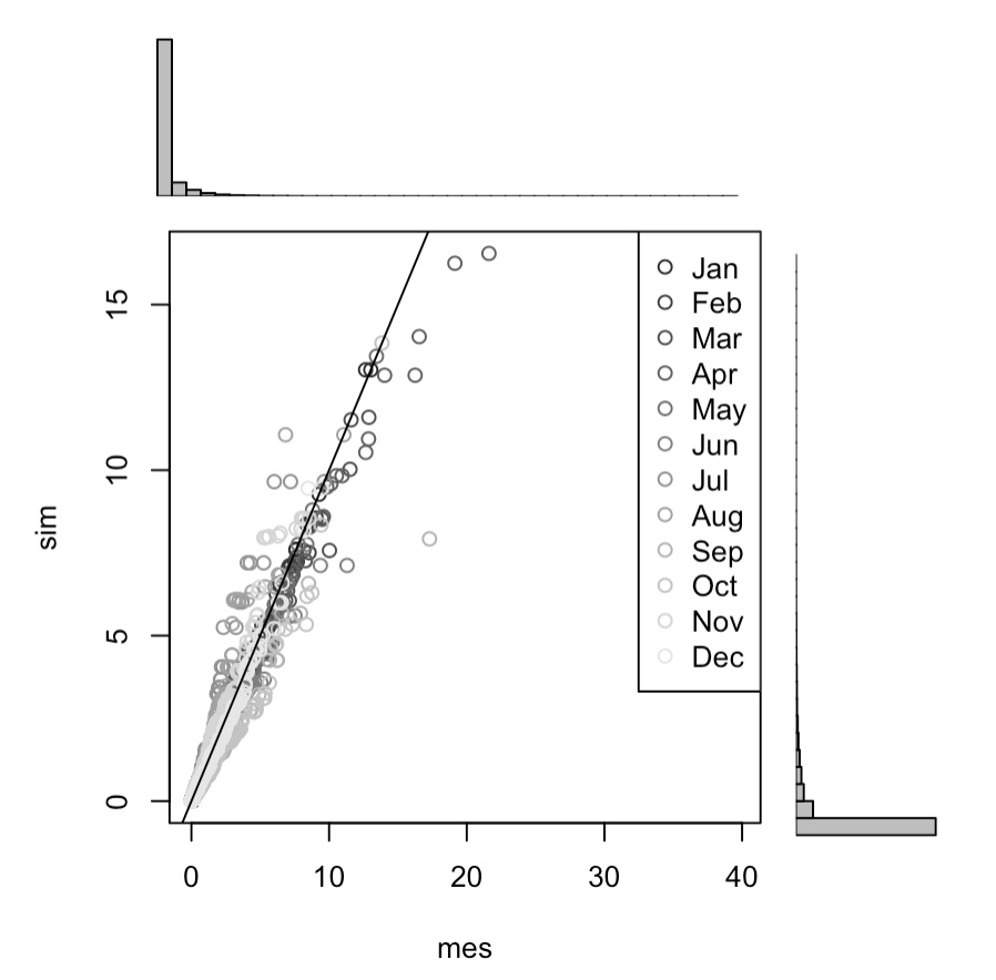
Figure 5.40: Comparison of monthly observed (ERA5) precipitation values with simulated ones. No systematic bias is visible.
5.4.2.4 Simulating Future Daily Climate
Using the insights gained so far, we can now generate future daily weather conditioned on the high resolution GCM output as described in the Section 5.4.1 above. For the climate impact assessment, we generate a 10-year mid 21st century run from 2051 - 2060 (called Period 1) and an end of 21st century run (2091 - 2100, Period 2) for both, the RCP 4.5 and RCP 8.5 concentration pathways. The climate scenarios will be compared to a baseline climate period from 2004 - 2013. These periods are specified in the following way in the parameters param list.
# Simulation periods
param$year_min_Baseline <- 2004
param$year_max_Baseline <- 2013
param$year_min_sim_Period1 <-  2051
param$year_max_sim_Period1 <-  2060
param$year_min_sim_Period2 <-  2091
param$year_max_sim_Period2 <-  2100
Now we are ready to prepare the climate scenarios14. The function riversCentralAsia::climateScenarioPreparation_RMAWGEN() prepares 2 climate scenarios between the years 2006 - 2100 where the user can define the periods of interest. Here, we want to investigate the 2 scenarios for the mid-21st century and the end of the century as defined above with the param$year_min_sim_Periodx and param$year_min_sim_Periodx parameters.
basin_climScen_Path <- './data/AmuDarya/GuntYashikul/ClimateProjections/'
basin_climScen_File <- 'climScen_monthly'

clim_scen <- climateScenarioPreparation_RMAWGEN(basin_climScen_Path,basin_climScen_File,param)
We have now defined the 12 precipitation and temperature scenarios, i.e. 2 for each RCP, 3 for each of the climate models available and 2 for each of the periods of interest, 2051 - 2060 and 2091-2100 and can rerun the stochastic weather generator while conditioning the scenarios on the mean future weather states.
# Compute for all stations
station_subset <- NULL # We compute climate projections for all subasin elevation bands.

# Return VAR model?
param$returnVARModel = FALSE

# Fire up the stochastic weather generator for all climate scenarios
PT_sim_all <- list()
# Loop through all climate scenarios and run models
for (idx in 1:length(clim_scen)){
  PT_sim_all[[idx]] <- wgen_daily_PT(param,station_data,station_subset,clim_scen[[idx]],param$returnVARModel)
}

names(PT_sim_all) <- names(clim_scen)
The PT_sim_all list contains the simulated daily minimum and maximum temperatures as well as precipitation values for the future periods of interest. In our case, these are the 10-year periods from 2051-2060 and 2091-2100 for all 3 available GCM models and the two RCPs. Summary statistics can be obtained for all scenarios and all stations with the riversCentralAsia::wgen_daily_summaryStats() function. This allows to carry out different types of top-level quick analyses for getting a good understanding of the future climate in the basin under consideration as a function of the target period and the GCM as well as the RCP. We show a couple of these analyses here.
First, all summary statistics are produced.
PT_sim_stats <- list()
for (idx in 1:length(clim_scen)){
  PT_sim_stats[[idx]] <-
    riversCentralAsia::wgen_daily_summaryStats(PT_sim_all[[idx]],param,station_data,station_subset,clim_scen[[idx]])
}
names(PT_sim_stats) <- names(clim_scen)
Before we show how to do some quick analyses, it should be remembered that we use the following definitions: - Baseline Period: 2004 - 2013; future Period 1: 2051 - 2060; and Future Period 2: 2091 - 2100.
For the station/elevation band Alishur_2, we get the following statistics of the daily climate projections under the GCM MIROC5 and RCP 45:
PT_sim_stats$rcp45_MIROC5_Period1$Alishur_2## P_baseline_obs P_futurePeriod_sim Tmin_baseline_obs
## Min. -1.153419e-14 -2.386486e-14 -33.087407
## 1st Qu. 1.472035e-02 1.137278e-02 -18.609744
## Median 1.179427e-01 1.044057e-01 -10.156870
## Mean 6.673150e-01 6.852445e-01 -10.885993
## 3rd Qu. 6.200780e-01 6.077338e-01 -2.393775
## Max. 3.974874e+01 2.368893e+01 8.173291
## Tmin_futurePeriod_sim Tmax_baseline_obs Tmax_futurePeriod_sim
## Min. -29.740110 -24.4808293 -20.340536
## 1st Qu. -15.362856 -7.2860936 -5.538543
## Median -7.659832 1.0043645 2.844080
## Mean -7.155001 0.3899992 3.561524
## 3rd Qu. 1.658264 8.4963461 13.508027
## Max. 14.897473 20.4007594 24.323957When comparing precipitation for the baseline period and the 2051 - 2060 period, the MIROC5 model suggests a slight increase of precipitation values in the Eastern Pamirs relative to the baseline (please note that the precipitation values in the table are in mm/day). At the same time, minimum mean temperatures are increasing from -10.89 degrees Celsius to -7.15 degrees Celsius, i.e. and increase of a remarkable 3.74 degrees. Our gut feeling tells us that this increase will be even more pronounced at the end of the 21st century and under RCP85. Let’s check!
First, we display the summary statistics for Alishur_2 of the GCM MIROC5 and the RCP45 for Period 2. As is visible in the table below, no significant changes are expected in terms of mean precipitation, also in Period 2 under this climate scenario and for this model. However, a further warming is expected where minimum mean temperatures increase to -6.38 degrees Celsius and and the mean maximum temperatures increase from 3.56 to 4.39 degrees Celsius. This suggests a pronounced winter warming.
PT_sim_stats$rcp45_MIROC5_Period2$Alishur_2## P_baseline_obs P_futurePeriod_sim Tmin_baseline_obs
## Min. -1.153419e-14 -3.214945e-14 -33.087407
## 1st Qu. 1.472035e-02 1.176385e-02 -18.609744
## Median 1.179427e-01 9.878187e-02 -10.156870
## Mean 6.673150e-01 6.881313e-01 -10.885993
## 3rd Qu. 6.200780e-01 5.786604e-01 -2.393775
## Max. 3.974874e+01 2.598245e+01 8.173291
## Tmin_futurePeriod_sim Tmax_baseline_obs Tmax_futurePeriod_sim
## Min. -31.997585 -24.4808293 -19.351808
## 1st Qu. -14.480643 -7.2860936 -4.926043
## Median -6.615511 1.0043645 3.641779
## Mean -6.379430 0.3899992 4.391877
## 3rd Qu. 1.938303 8.4963461 14.078694
## Max. 15.692796 20.4007594 27.346588Finally, we do the same for this station/elevation band using the GCM MIROC5 and the RCP85 for Period 2.
PT_sim_stats$rcp85_MIROC5_Period2$Alishur_2## P_baseline_obs P_futurePeriod_sim Tmin_baseline_obs
## Min. -1.153419e-14 -4.613131e-14 -33.087407
## 1st Qu. 1.472035e-02 1.446667e-02 -18.609744
## Median 1.179427e-01 1.274579e-01 -10.156870
## Mean 6.673150e-01 8.162968e-01 -10.885993
## 3rd Qu. 6.200780e-01 6.999277e-01 -2.393775
## Max. 3.974874e+01 2.861400e+01 8.173291
## Tmin_futurePeriod_sim Tmax_baseline_obs Tmax_futurePeriod_sim
## Min. -27.939768 -24.4808293 -16.552664
## 1st Qu. -11.924017 -7.2860936 -2.694583
## Median -4.036578 1.0043645 6.522826
## Mean -3.175482 0.3899992 7.111490
## 3rd Qu. 6.167460 8.4963461 17.411537
## Max. 19.289063 20.4007594 29.213902It can easily be seen that our intuition from above is correct and that the modeling results for example suggest a 7.71 degrees warming of the minimum mean temperatures over this period. At the same time, the model suggests that mean precipitation is slightly increasing from approx. 245 mm/year to 298 mm/year. This corresponds to an increase of approx. 22 % relative to the baseline.
With a projected mean precipitation of 332 mm/year (increase of approx. 36 % relative to baseline), the GCM ACCESS1_3 projects the most pronounced increase in precipitation for Alishur_2 under the RCP85 for the period 2091-2100. The GCM CMCC_CM even suggests a slight decrease of total annual precipitation relative to the baseline. While precipitation projections of GCMs are notoriously uncertain, one relatively robust conclusion to make is that precipitation levels are expected to stay at the current levels or slightly increase. All these findings now require us to study with great care implications on the hydrology of the river basins in the region.
PT_sim_stats$rcp85_ACCESS1_3_Period2$Alishur_2## P_baseline_obs P_futurePeriod_sim Tmin_baseline_obs
## Min. -1.153419e-14 -6.337539e-14 -33.087407
## 1st Qu. 1.472035e-02 1.072765e-02 -18.609744
## Median 1.179427e-01 9.955763e-02 -10.156870
## Mean 6.673150e-01 9.109544e-01 -10.885993
## 3rd Qu. 6.200780e-01 6.344134e-01 -2.393775
## Max. 3.974874e+01 5.413337e+01 8.173291
## Tmin_futurePeriod_sim Tmax_baseline_obs Tmax_futurePeriod_sim
## Min. -28.262056 -24.4808293 -15.105202
## 1st Qu. -12.339332 -7.2860936 -1.919159
## Median -5.582341 1.0043645 5.690707
## Mean -4.861328 0.3899992 6.521103
## 3rd Qu. 3.320528 8.4963461 15.812779
## Max. 14.406063 20.4007594 26.480914PT_sim_stats$rcp85_CMCC_CM_Period2$Alishur_2## P_baseline_obs P_futurePeriod_sim Tmin_baseline_obs
## Min. -1.153419e-14 -4.463575e-14 -33.087407
## 1st Qu. 1.472035e-02 9.058688e-03 -18.609744
## Median 1.179427e-01 7.933737e-02 -10.156870
## Mean 6.673150e-01 6.559270e-01 -10.885993
## 3rd Qu. 6.200780e-01 4.975115e-01 -2.393775
## Max. 3.974874e+01 2.489362e+01 8.173291
## Tmin_futurePeriod_sim Tmax_baseline_obs Tmax_futurePeriod_sim
## Min. -28.453681 -24.4808293 -16.855502
## 1st Qu. -9.314596 -7.2860936 -1.298192
## Median -1.021698 1.0043645 6.787816
## Mean -1.957580 0.3899992 7.465019
## 3rd Qu. 5.594001 8.4963461 16.946780
## Max. 16.520962 20.4007594 28.491711For this purpose, we convert these daily climatologies into hourly ones and export them as scenario files that can be read into RS MINERVE where we can perform hydrological scenario analysis. The downscaling to hourly values as well as the exporting is shown in the Section below.
5.4.2.5 Exporting Climate Scenarios as .csv-files for import in RS MINERVE
For exporting to RS MINERVE, a .csv file needs to be generated very much alike the one described in Section 5.3.2.4. Prior to exporting such scenario-dependent files, we need to generate hourly time series from the daily simulated ones. To do this, different approaches are chosen for the precipitation values as well as the temperature time series. The conversion can automatically be done with the helper function riversCentralAsia::generateHourlyFromDaily_PT() that accepts the daily climate scenarios as variable from which it downscales to hourly data and prepares the tabular export as .csv-file for later import in RS MINVERVE.
As for total daily precipitation [mm/day], it is available for each day for the future periods of interest and for each station/elevation band. riversCentralAsia::generateHourlyFromDaily_PT() converts these values by uniformly distribution the total daily precipitation over the 24 hours within one day, i.e. from 00:00:00 to 23:00:00. More details on this can be found in the help section of the function.
For temperature, the challenge is a bit bigger since we ideally would want to take into account the diurnal cycle of temperature to vary between the daily minimum and maximum temperatures characteristically. How to get the diurnal cycle for the stations/elevation bands?
What is being proposed here is to use the hourly ERA5 data over the baseline period and to extract a mean dirurnal cycle for each station there measured over all baseline period observation days. Under the assumption that these station cycles remain the same in the future, they are adjusted for each day so that minimum and maximum daily temperatures from the climate scenarios correspond to minimum and maximum diurnal cycle values. As is shown below, the function riversCentralAsia::computeDiurnalTemperatureCycle() computes these diurnal station cycles.
filePath <- './data/AmuDarya/GuntYashikul/RSMinerve/'
fileName <- 'Gunt_Yashikul_1981_2013_db.csv'
era5_gunt_yashikul <- read.table(paste0(filePath,fileName),sep=',') %>% as_tibble()

# Subcatchment suspects to delete because we do not use them in the RR Model
idx2del <- (era5_gunt_yashikul[1,]=='Gunt_DS_1')|(era5_gunt_yashikul[1,]=='Gunt_DS_2')|
  (era5_gunt_yashikul[1,]=='Gunt_DS_3')
era5_gunt_yashikul <- era5_gunt_yashikul %>% dplyr::select(which(!idx2del))

# Compute diurnal cycle
diurnalCycle <- computeDiurnalTemperatureCycle(era5_gunt_yashikul,param)

# Simple visualization
diurnalCycle %>% pivot_longer(-hour) %>% group_by(name) %>%
  ggplot(.,aes(x=hour,y=value,colour=name)) + geom_line() + labs(title="ERA5 Diurnal T Variation, Gunt-Yashikul River Subbasins")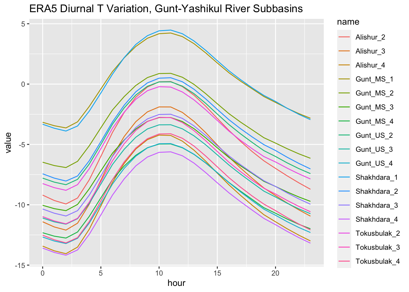
Using riversCentralAsia::generateHourlyFromDaily_PT(), the daily climate scenario files can be produced in a very simple manner.
# Producing the hourly climate scenarios
climScen_hourly <- generateHourlyFromDaily_PT(PT_sim_all,era5_gunt_yashikul,param)
# Adding the required header information to the data frames for each climate scenario
headerRows<- era5_gunt_yashikul[1:8,] %>% dplyr::select(-which(era5_gunt_yashikul[5,]=='Q'))
climScen_hourly_rsminerve <- list()
for (idx in 1:length(climScen_hourly)){
  climScen2Export <- climScen_hourly[[idx]] %>% mutate(across(everything(), as.character))
  names(climScen2Export) <- names(headerRows)
  climScen_hourly_rsminerve[[idx]] <- headerRows %>% add_row(climScen2Export)
}
names(climScen_hourly_rsminerve) <- names(clim_scen)
Now, finally, we can store these files as climate scenario files on the disk for later importing into RS MINERVE.
outputPath <- './data/AmuDarya/GuntYashikul/RSMinerve/' # Specify the output path of the files
names2Save <- names(climScen_hourly_rsminerve) # Specification of the file names (do not change)
names2Save_prefix <- 'Gunt_Yashikul_' # Change according to the basin that you are working with
for (idx in 1:length(climScen_hourly_rsminerve)){
  fileName <- paste0(names2Save_prefix,names2Save[idx],'.csv')
  write.table(climScen_hourly_rsminerve[[idx]],
              paste0(outputPath,fileName),sep=',',
              row.names = FALSE,col.names=FALSE,
              quote=FALSE,append=FALSE)
}
This is the same algorithm that was used to produce high-resolution reanalysis data as discussed in Chapter @ref(Data::ClimateReanalysisData).↩︎
If you download these data, it is advisable to maintain the directory structure as given via the Dropbox link. Please note that the entire directory is 4.79 GB of data.↩︎
Detailed information about the core functions of RMAWGEN can be obtained by consulting their help, i.e. by for example typing
?ComprehensivePrecipitationGenerator.↩︎The prepared monthly climate scenarios of this RS MINVERVE model can be found in this directory
'./data/AmuDarya/GuntYashikul/ClimateProjections/'. Since RMAWGEN requires precipitation, mean minimum and mean maximum temperature on a monthly basis, these data are prepared using the functionriversCentralAsia::climateScenarioPreparation_RMAWGEN()for the periods of interest in the future.↩︎