3.1 Gunt River Basin
3.1.1 Basin Characterization
The Gunt river basin is located in the Pamir mountains in the Gorno Badakhshan Autonomous Region in south-east Tajikistan. The basin covers approximately 14’000 km2. The Gunt river is a large right tributary of the upstream Pyandzh and joins the latter downstream of the town of Khorog. Mean elevation is approx 4’270 meters above mean sea level (masl) with a pronounced altitude range from 2’000 – 6’700 masl. The highest elevations in the catchment are Peak Karl Marx (6726 m) and Peak Engels (6510 m) at the southern border of the catchment. A map of the basin is provided in Figure 3.1.
# convert to sf object
meteoStations_sf <- st_as_sf(meteoStations %>% dplyr::select(StationName,lat,lon),
                            coords = c("lon","lat"),
                            remove = FALSE,
                            crs = "epsg:32642",
                            agr = "constant")

# Load catchment shp
gunt_Shapefile <- st_read('./data/AmuDarya/Gunt/GeospatialData/Gunt_Basin_poly.shp',quiet = TRUE)
gunt_Shapefile <- gunt_Shapefile %>% subset(fid==2)
gunt_Shapefile_LatLon <- st_transform(gunt_Shapefile,crs = st_crs(4326))
areaGunt <- gunt_Shapefile %>% st_area() %>% as.numeric()
# Load subbasins
gunt_subbasins_shp <- st_read('./data/AmuDarya/Gunt/GeospatialData/Gunt_Subbasins_RSMinerve.shp',quiet = TRUE)

# Areas of Interest
aoi_CentralAsia_LatLon <- extent(c(65,80.05,35.95,44.05)) # in lat/lon
aoi_Basin_LatLon <- gunt_Shapefile_LatLon %>% extent() # GUNT
aoi_Basin_UTM <- gunt_Shapefile %>% extent() # GUNT, in UTM

# Load DEM
Gunt_DEM <- raster('./data/AmuDarya/Gunt/GeospatialData/17050_Gund_Basin_DEM.tif')
Gunt_DEM_lr <- raster::aggregate(Gunt_DEM,fact=10) # this is in UTM 42N
Gunt_DEM_lr_LatLon <- raster::projectRaster(Gunt_DEM_lr, crs = "+init=epsg:4326")

# Load simplified river network with first order tributaries only
gunt_river_shape <- st_read('./data/AmuDarya/Gunt/GeospatialData/Gunt_Rivers_RSMinerve.shp',quiet = TRUE)

# Create slope and hillshade
slope = terrain(Gunt_DEM_lr_LatLon, opt='slope')
aspect = terrain(Gunt_DEM_lr_LatLon, opt='aspect')
hillshade_Gunt = hillShade(slope, aspect, 40, 270)

# Subbasins naming
subbasins <- # just put everything in a regular dataframe
  tibble(basin=c("Shakhdara","Gunt","Tokusbulak","Alishur"),
         lat   = c(37.2,37.75,37.6,37.61),
         lon   = c(72.0,71.8,72.6,73.25))
subbasins_coord_latlon = SpatialPoints(cbind(subbasins$lon, subbasins$lat), proj4string=CRS("+proj=longlat"))
subbasins_coord_UTM <- spTransform(subbasins_coord_latlon, CRS("+init=epsg:32642")) %>%
  coordinates() %>% as_tibble() %>%
  rename(x=coords.x1,y=coords.x2)
subbasins <- bind_cols(subbasins,subbasins_coord_UTM)

# Convert to dataframe for ggplotting
Gunt_DEM_spdf <- as(Gunt_DEM_lr_LatLon, "SpatialPixelsDataFrame")
Gunt_DEM_df <- as.data.frame(Gunt_DEM_spdf)
colnames(Gunt_DEM_df) <- c("value", "x", "y")
hillshade_Gunt_spdf <- as(hillshade_Gunt, "SpatialPixelsDataFrame")
hillshade_Gunt_df <- as.data.frame(hillshade_Gunt_spdf)
colnames(hillshade_Gunt_df) <- c("value", "x", "y")

# plot
ggplot() +
  geom_tile(data = hillshade_Gunt_df, aes(x = x, y = y, fill = value)) +
  scale_fill_gradient(low = "black", high = "white") +
  new_scale_fill() +
  geom_tile(data=Gunt_DEM_df, aes(x=x, y=y, fill=value), alpha=0.8)+
  geom_sf(data=gunt_Shapefile_LatLon,color="black",fill=NA) +
  geom_sf(data=gunt_subbasins_shp,color="black",fill=NA,linetype="11",size=0.25) +
  geom_sf(data=gunt_river_shape,color="blue",fill=NA) +
   geom_point(data = meteoStations,
                aes(x = lon, y = lat),
                size = 2, shape = 23,
                fill = "darkred") +
   geom_text(data = meteoStations,
               aes(x = lon, y = lat, label = StationName),
               vjust = -.3,
               hjust = -.2) +
  scale_fill_gradientn(colours = terrain.colors(100)) +
  xlab("Longitude") + ylab("Latitude") +
  guides(fill=guide_legend(title="Alt. [masl]")) +
  # ggtitle("Gunt Catchment with Main Subbasins") +
  coord_sf(xlim = c(71.4, 74.2), ylim = c(36.9, 38.2), expand = FALSE)  +
  geom_label(data = subbasins,aes(x = lon, y = lat, label = basin),vjust = 0,hjust = 0)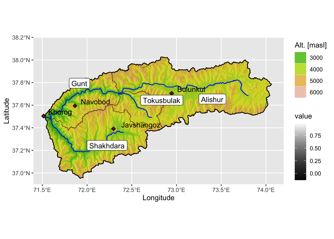
Figure 3.1: Map of the Gunt river basin. The subcatchments are named with white labels and the meteorological stations indicated with red diamonds. The discharge station 17050 at Gunt is located at the meteostation 38954.
The river emerges as Alishur river in the Easter Pamir Plateau and the flows west through the western Pamirs before joining Pyandzh. The Eastern Pamirs is a high plateau located above 4’000 masl. The Western Pamirs are occupied by high mountain ranges separated from each other by deep valleys (see (Odinaev 2021) and citations therein for more information). Alishur river is named Gunt river after exiting lake Yashikul. Gunt river has two main tributaries, i.e. the Tokusbulak river and the Shakhdara river (see again Figure 3.1.
One discharge gauging station exists which has a near complete monthly measurement record from 1940 onward. The data are shown in Figure 3.2. More details on these data is presented in the Section 3.1.2. The available meteorological station data is discussed in Section 3.1.3. The station characteristics are summarized in the following Table.
## MeteoStation locations and elevation
meteoStations <- # just put everything in a regular dataframe
  tibble(StationName=c("Bulunkul","Khorog","Khorog","Javshangoz","Navobod"),
         StationCode = c(38953, 38954, 17050, 38956, 38950),
         lat   = c(37.70416667,37.50361111,37.50361111,37.39083333,37.59416667),
         lon   = c(72.94583333,71.515,71.515,72.29583333,71.86555556),
         utm.x = NA,
         utm.y = NA,
         masl  = c(3746, 2075, 2075,3438, 2566),
         type = c("Meteo", "Meteo","Discharge Gauge","Meteo","Meteo"))
## convert lat / lon coordinates to UTM
cord.dec = SpatialPoints(cbind(meteoStations$lon, meteoStations$lat), proj4string=CRS("+proj=longlat"))
cord.UTM <- spTransform(cord.dec, CRS("+init=epsg:32642"))
cord.UTM.tbl <- cord.UTM %>% as_tibble()
meteoStations$utm.x <- cord.UTM.tbl$coords.x1
meteoStations$utm.y <- cord.UTM.tbl$coords.x2
meteoStations
## # A tibble: 5 x 8
## StationName StationCode lat lon utm.x utm.y masl type
## <chr> <dbl> <dbl> <dbl> <dbl> <dbl> <dbl> <chr>
## 1 Bulunkul 38953 37.7 72.9 847891. 4180325. 3746 Meteo
## 2 Khorog 38954 37.5 71.5 722309. 4153714. 2075 Meteo
## 3 Khorog 17050 37.5 71.5 722309. 4153714. 2075 Discharge Gauge
## 4 Javshangoz 38956 37.4 72.3 791785. 4143330. 3438 Meteo
## 5 Navobod 38950 37.6 71.9 752995. 4164650. 2566 MeteoThe Table below summarizes key basin statistics that are relevant from the hydro-climatological perspective. Data from various sources are summarized here. The basin area has been derived from the basin shapefile. Raster statistics of the SRTM digital elevation model ((“Srtmgl1 n -ASA SRTM Version 3.0” 2020b)), the climate raster files as well as the land cover raster are calculated using the QGIS Raster Layer Statistics processing toolbox algorithm. The land ice total polygon area is computed with the Statistical Summary Option in QGIS.
The norm hydrological year discharge and the corresponding norm cold and warm season discharge values have been computed with data from the Tajik Hydrometeorological Service. The mean basin precipitation is computed using a state-of-the-art bias corrected reanalysis product (Beck et al. 2020a). Such data will also be used for hydro-climatological modeling in later Chapters (also see Chapter 5 for more information on data products). Potential evaporation is from (Trabucco and Zomer 2019) using the Penman-Montieth equation.
| ATTRIBUTE | VALUE |
|---|---|
| Geography (“Srtmgl1 n -ASA SRTM Version 3.0” 2020b) | |
| Basin Area \(A\) | 13’693 km2 |
| Minimum Elevation \(h_{min}\) | 2’068 masl |
| Maximum Elevation \(h_{max}\) | 6’652 masl |
| Mean Elevation \(h_{mean}\) | 4’267 masl |
| Hydrology [Source: Tajik Hydromet Service] | |
| Norm hydrological year discharge \(Q_{norm}\) | 103.8 m3/s |
| Norm cold season discharge (Oct. - Mar., Q4/Q1) | 19.8 m3/s |
| Norm warm season discharge (Apr. - Sept., Q2/Q3) | 84.2 m3/s |
| Annual norm discharge volume | 3.28 km3 |
| Annual norm specific discharge | 239 mm |
| Climate | |
| Mean basin temperature \(T\) (Karger et al. 2017) | -5.96 deg. Celsius |
| Mean basin precipitation \(P\) (Beck et al. 2020a) | 351 mm |
| Potential Evaporation \(E_{pot}\) (Trabucco and Zomer 2019) | 929 mm |
| Aridity Index \(\phi = E_{pot} / P\) | 2.7 |
| Aridity Index (Trabucco and Zomer 2019) | 3.6 |
| Land Cover (Buchhorn et al., n.d.) | |
| Shrubland | 8 km2 |
| Herbaceous Vegetation | 4’241 km2 |
| Crop Land | 0.5 km2 |
| Built up | 4 km2 |
| Bare / Sparse Vegetation | 8’410 km2 |
| Snow and Ice | 969 km2 |
| Permanent Water Bodies | 80 km2 |
| Land Ice | |
| Total glacier area (GLIMS and NSIDC 2005) | 875 km2 |
| Total glacier volume (calculated with (Erasov 1968)) | 699 km3 |
With the values provided in the table above, the discharge index \(Q/P\) is 68.5 % and the evaporative index \(E/P\) is 31.5 %. In other words, the long-term water balance shows that 3 precipitation units gets partitioned into 2 discharge units and 1 evaporation unit, approximately. The aridity index \(\phi\) , when calculated using \(P\) from (Beck et al. 2020a) and \(E_{pot}\) from (Trabucco and Zomer 2019) is 2.7. The aridity index from (Trabucco and Zomer 2019) is 3.6. These values indicate some uncertainty in relation to these global clmiate products used. Despite this, they confirm the highly arid characteristics of the basin.
3.1.2 Hydrology
For the analysis of the key hydro-climatological characteristics, we first load the available decadal and monthly station data4. The data used in this Chapter can be accessed on the public GitHub repository Applied Modeling of Hydrological Systems in Central Asia and the ./data/AmuDarya/Gunt/ folder in there.
First, we load the available data into R.
# Load data records
fPath = fPath <- './data/AmuDarya/Gunt/StationData/'
fName = 'gunt_data_cleaned.Rds'
data <- read_rds(paste0(fPath,fName))
data
## # A tibble: 23,352 x 10
## date data norm units type code station river basin resolution
## <date> <dbl> <dbl> <chr> <chr> <chr> <chr> <chr> <chr> <fct>
## 1 1940-01-31 30.5 32.9 m3/s Q 17050 Gunt_Khorog Gunt Pyandz mon
## 2 1940-02-29 27.3 30.1 m3/s Q 17050 Gunt_Khorog Gunt Pyandz mon
## 3 1940-03-31 24.9 28.4 m3/s Q 17050 Gunt_Khorog Gunt Pyandz mon
## 4 1940-04-30 26.4 30.7 m3/s Q 17050 Gunt_Khorog Gunt Pyandz mon
## 5 1940-05-31 59 68.5 m3/s Q 17050 Gunt_Khorog Gunt Pyandz mon
## 6 1940-06-30 309 232. m3/s Q 17050 Gunt_Khorog Gunt Pyandz mon
## 7 1940-07-31 224 319. m3/s Q 17050 Gunt_Khorog Gunt Pyandz mon
## 8 1940-08-31 201 237. m3/s Q 17050 Gunt_Khorog Gunt Pyandz mon
## 9 1940-09-30 121 117. m3/s Q 17050 Gunt_Khorog Gunt Pyandz mon
## 10 1940-10-31 60.8 63.1 m3/s Q 17050 Gunt_Khorog Gunt Pyandz mon
## # … with 23,342 more rowsThis dataframe contains all available data hydro-meteorological data from the basin. All available hydro-meteorological stations in the basin are listed in the following dataframe were defined above.
Most data are available at monthly time scales. The discharge data from Gauge 17050 can be accessed and extracted from the Gunt dataset in the following way.
q_17050_mon <- data %>% filter(type == "Q" & code == '17050' & resolution == 'mon')
q_17050_mon
## # A tibble: 972 x 10
## date data norm units type code station river basin resolution
## <date> <dbl> <dbl> <chr> <chr> <chr> <chr> <chr> <chr> <fct>
## 1 1940-01-31 30.5 32.9 m3/s Q 17050 Gunt_Khorog Gunt Pyandz mon
## 2 1940-02-29 27.3 30.1 m3/s Q 17050 Gunt_Khorog Gunt Pyandz mon
## 3 1940-03-31 24.9 28.4 m3/s Q 17050 Gunt_Khorog Gunt Pyandz mon
## 4 1940-04-30 26.4 30.7 m3/s Q 17050 Gunt_Khorog Gunt Pyandz mon
## 5 1940-05-31 59 68.5 m3/s Q 17050 Gunt_Khorog Gunt Pyandz mon
## 6 1940-06-30 309 232. m3/s Q 17050 Gunt_Khorog Gunt Pyandz mon
## 7 1940-07-31 224 319. m3/s Q 17050 Gunt_Khorog Gunt Pyandz mon
## 8 1940-08-31 201 237. m3/s Q 17050 Gunt_Khorog Gunt Pyandz mon
## 9 1940-09-30 121 117. m3/s Q 17050 Gunt_Khorog Gunt Pyandz mon
## 10 1940-10-31 60.8 63.1 m3/s Q 17050 Gunt_Khorog Gunt Pyandz mon
## # … with 962 more rowsWhen we plot the data, we see that we have a near complete monthly record from 1940 onward (Figure 3.2). The data gap in the 1990ies was during the Tajik civil war.
q_17050_mon %>% plot_time_series(date,
                                 data,
                                 .smooth        = FALSE,
                                 .interactive   = TRUE,
                                 .title         = "",
                                 .x_lab         = 'Year',
                                 .y_lab         = 'Mean monthly Q [m3/s]',
                                 .plotly_slider = TRUE)
Figure 3.2: Monthly Discharge Data at Gunt Gauging Station (17050)
The visible changes in the low flow regime from 2007 onward are because of starting man-made regulations of the low-flow winter discharge regime for the generation of winter hydropower electric energy in the newly constructed facility in Khorog. When hydropower is required, the water table of the natural lake Yashikul in the Pamir plateau gets lowered to increase the discharge for energy production.
knitr::include_graphics('./_bookdown_files/FIG_FOREWORD/Yashikul_PamirEnergy_Final.jpg')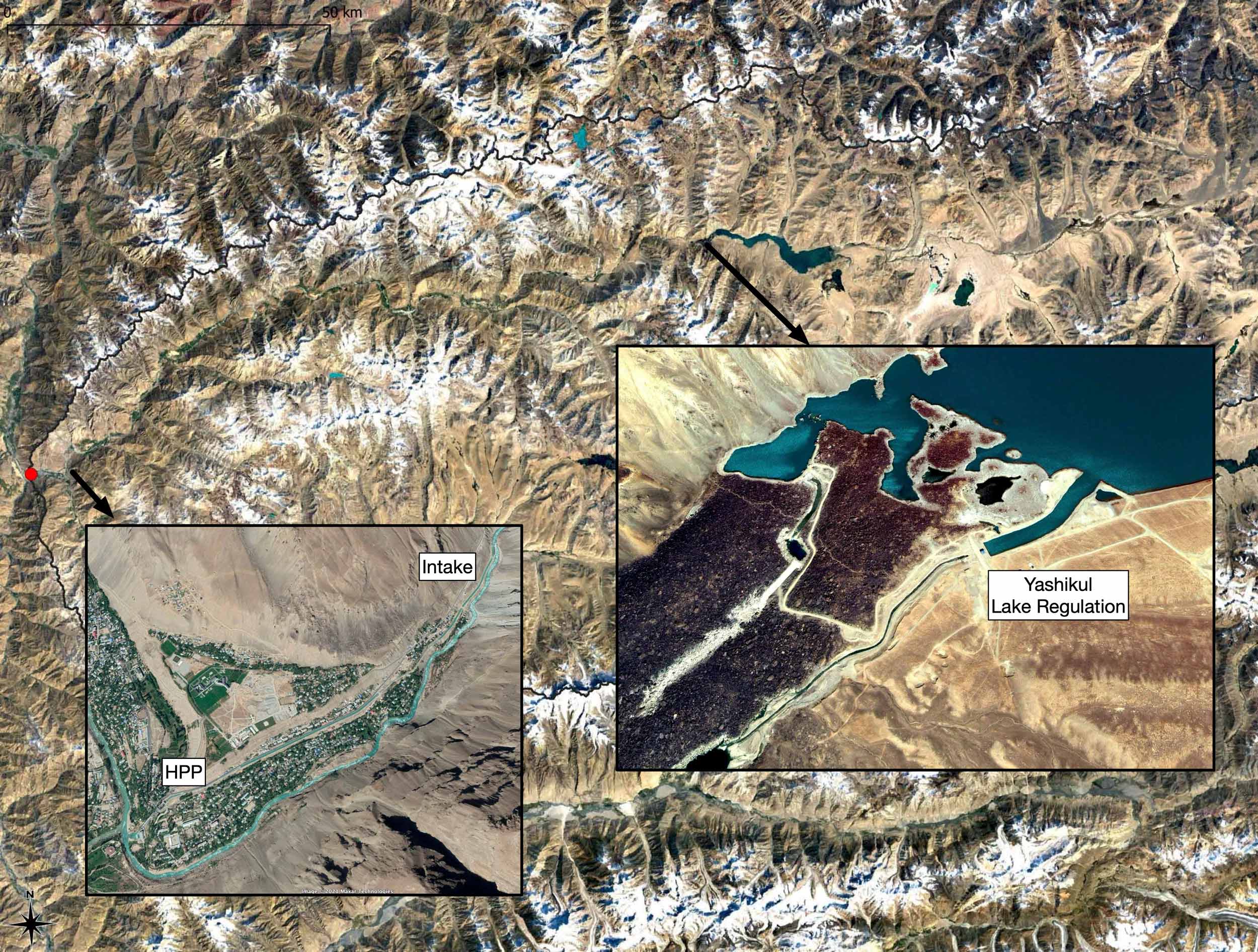
Figure 3.3: Since 2006, a run off the river hydropower plant operated by Pamir Energy produces hydropower to cover local electric energy demand. Lake Yashikul is used as a regulator. The increase in winter discharge from 2007 onwards is due to HPP operations.
The seasonal diagnostics of the monthly discharge time series is shown in Figure 3.4. The peak discharge of Gunt river measured at Khorog station is in July.
q_17050_mon %>%
  plot_seasonal_diagnostics(.date_var      = date,
                            .value         = data,
                            .title         = "",
                            .feature_set   = c("month.lbl"),
                            .interactive   = FALSE,
                            .x_lab         = "Year",
                            .y_lab         = "Mean monthly Q [m3/s]") +
  scale_x_discrete(breaks=c("January", "February", "March", "April", "May",
                            "June", "July", "August", "September", "October",
                            "November", "December", "1", "2", "3", "4"),
                   labels=c("J", "F", "M", "A", "M", "J", "J", "A", "S", "O", "N", "D","1", "2", "3", "4"))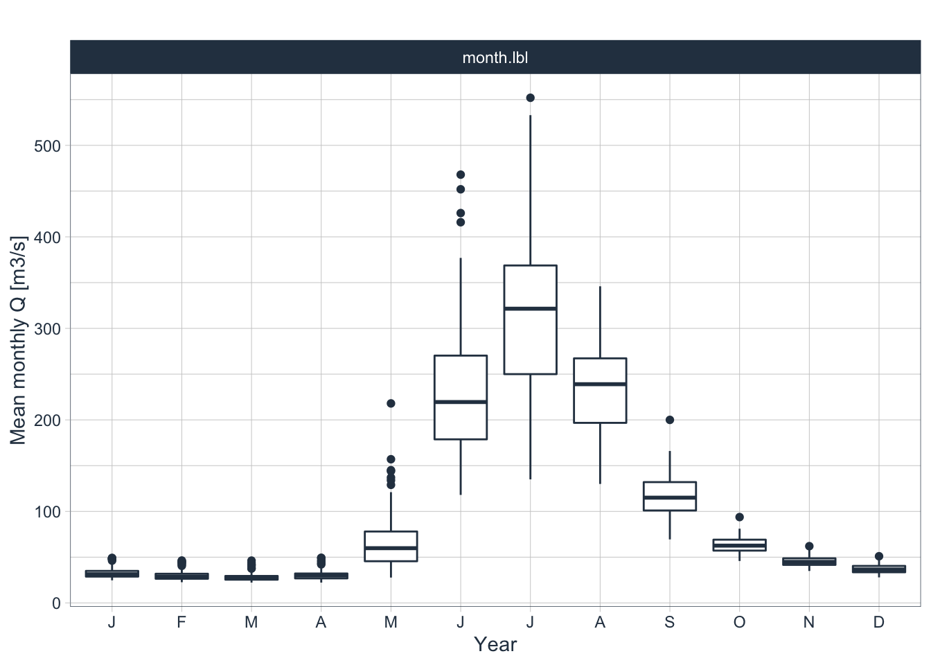
Figure 3.4: Seasonal diagnostics of the monthly discharge time series at the Gunt-Khorog gauging station (17050)
unlike in the lower lying Chirchik tributaries as shown in Figure 3.15 above.
E3.1
Peak Discharge
Discuss with your colleague(s):
- Compare discharge seasonality with the seasonality of the large Chirchik River tributaries?
- Obtain the information of all the other rivers in the Case Study packs and their seasonality.
- What is the single most important determinant of peak discharge timing in Central Asia rivers?
Below in Figure ??, we are plotting changes to monthly flows over time by binning all available data in the corresponding monthly slots. The red lines are linear regression lines that indicate trends for the individual months. Over the observational record of approx. 80 years, changes in monthly discharge regimes are clearly visible. On the one hand, summer discharge of Gunt river during the third quarter (Q3) is decreasing whereas the cold season discharge in Q1 and Q4 is increasing. This is a clear indication that the basin hydrology is already reacting to a changing climate. This is one of the observations that motivates us to further investigate future changes with hydrological modeling (see Chapter 6 and (Odinaev 2021) for more details).
q_17050_mon %>%
  summarise_by_time(.date_var = date,
                    .by       = "month",
                    value     = mean(data)) %>%
  tk_ts(frequency = 12) %>%
  forecast::ggsubseriesplot(year.labels = FALSE) +
              geom_smooth(method = "lm",color="red") +
              xlab('Month') +
              ylab('Mean monthly Q [m3/s]')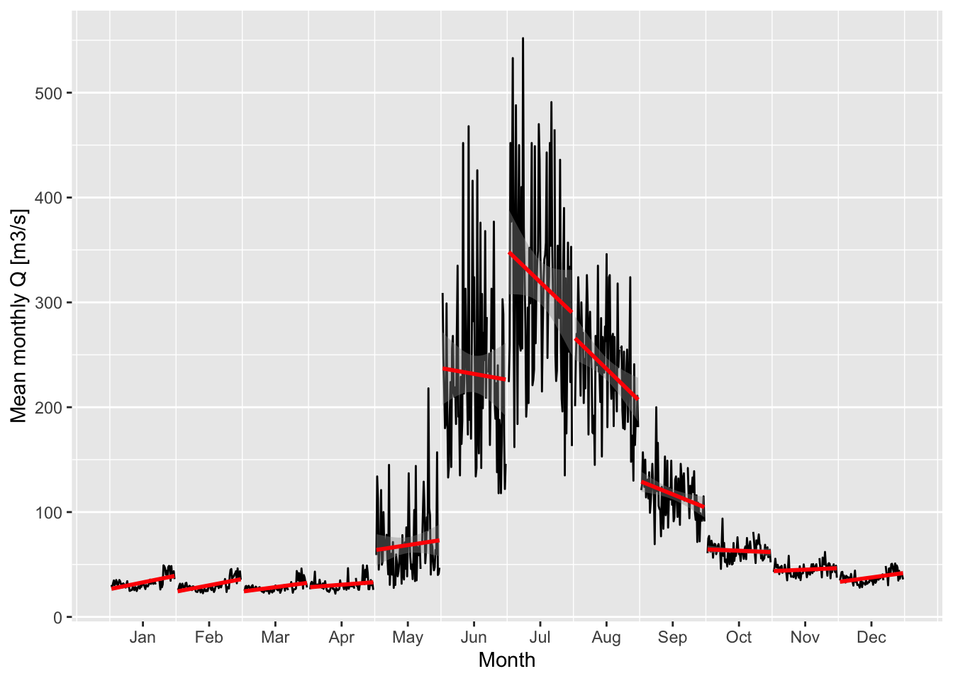
Whenever we analyze annual data and changes therein, we should work with data as observed during the hydrological year. The hydrological year in Central Asia is defined as:
monHY(Oct) = 1
monHY(Nov) = 2
…
monHY(Sep) = 12
This also holds for meteorological data. Using this definition, we can further define cold and warm seasons easily where the cold season lasts from October through end of March (Q4 to Q1 the following year) and the warm season from April through end of September (Q2 and Q3). With this in mind, we can define the hydrological year discharge.
The function convert2HYY() as part of the riversCentralAsia package provides a convenient way to compute hydrological year mean discharge, including for cold and warm seasons. For monthly mean temperatures mean(T), it computes hydrological year mean temperatures, including for cold and warm seasons. Finally, for precipitation, the function computes the hydrological year sum, including also for cold and warm season months. Figure 3.5 shows the discharge time series analysis for the Khorog gauging station.
# Computation of hydrological year discharge and plotting
qHYY <- data %>% convert2HYY(.,'17050','Q')
qHYY %>%   pivot_longer(-hyYear) %>%
  plot_time_series(hyYear,value,name,
                   .title = '',
                   .x_lab = 'Year',
                   .y_lab = 'Mean monthly Q [m3/s]',
                   .interactive = FALSE,
                   .smooth=FALSE)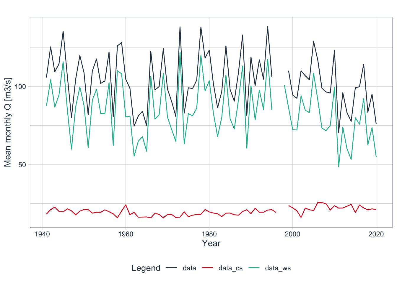
Figure 3.5: Hydrological year discharge timeseries, incl. cold and warm season values. If data are not complete for all 12 months, the hydrological year statistics are not computed. data: entire year discharge, data_cs: cold season Q1/Q4 discharge and data_ws: warm season Q2/Q3 discharge.
Figure 3.5 confirms the findings from the seasonal analysis. However, it also shows that the first two decades of the 21st century show a marked decline in total discharge as compared to the period between 1960 to 2000.
A common way to plot changes over time in hydrometeorological time series is to plot annual deviations from corresponding long-term norms (long-term mean values). For this, we can use the plotNormDevHYY() function. Given the three hydrological year annual time series, it computes long-term norms over the entire data set and subtracts actual annual values from the norm value. Like this, temporal changes and trends become even better visible. Figure 3.6 shows the results for the hydrological year data shown in Figure 3.5.
plotNormDevHYY(qHYY,'Q','Khorog-Gunt 17050')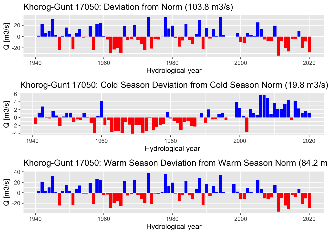
Figure 3.6: Deviations from the corresponding long-term norms for the discharge time series at gauging station 17050. It should be noted that the values shown are deviations from the corresponding norms which are shown in the subtitles above the figure plates.
Figure 3.6 shows that in absolute terms, the discharge in the high-flow season is undergoing a much greater reduction than an increase in the low-flow season. Hence, we cannot simply explain the decline of discharge in one season with the increase in the other. In other words, the early melting of the winter snow pack cannot alone explain the summer decline in water availability. Some other mechanism much be at work which we still need to better understand. One hypothesis could be that an increase in summer temperatures leads to higher evaporation over the basin thus leading to reduced discharge (see also Section ?? below).
Also and as mentioned above, winter discharge is influence by human regulation from 2006 onward. This needs to be carefully taken into account when carrying out climate change impact analysis over the period of the observational record. For example, the cold season discharge deviation from the norm in 2006 and 2007 is 6 m3/s (see Figure 3.6) indicating that this amount of additional water was used for hydropower energy production.
In order to gauge whether there is a robust trend in discharge over the observed time period, we compute decadal (10 year means) and plot the results.
mean10yearQ <- qHYY %>% filter(hyYear < '2020-01-01') %>%
  pivot_longer(-hyYear) %>% group_by(name) %>% summarise_by_time(hyYear,value,.by="10 year",mean10yearQ = mean(value,na.rm=TRUE)) %>% dplyr::select(-value) %>% distinct() %>% ungroup()
mean10yearQ %>% pivot_wider(names_from = name,values_from = mean10yearQ)
## # A tibble: 8 x 4
## hyYear data data_cs data_ws
## <date> <dbl> <dbl> <dbl>
## 1 1940-01-01 111. 20.1 91.1
## 2 1950-01-01 108. 19.4 88.6
## 3 1960-01-01 96.2 17.8 78.4
## 4 1970-01-01 105. 17.9 86.9
## 5 1980-01-01 105. 18.7 85.8
## 6 1990-01-01 114. 20.5 93.9
## 7 2000-01-01 104. 21.9 82.6
## 8 2010-01-01 94.2 22.3 71.9mean10yearQ %>% plot_time_series(hyYear,mean10yearQ,name,
.smooth = FALSE,
.x_lab = "Year",
.y_lab = "Q [m^3/s]",
.title = "")Figure 3.7: 10-year mean hydrological year discharge of Gunt River, including the cold and warm season components. The decadal mean values are related in time to the beginning of the corresponding decade in the Figure. The strongly declining trend in warm season discharge causes the overall observed decline in hydrological year discharge.
This is informative. From the 1990ies onwards, a strong reduction in mean hydrological year warm season discharge is observed of about - 16% relative to mean 1940 - 1989 values. At the same time, 10-year mean hydrological year cold season discharge remained almost stable. As already mentioned, these findings are the a key motivation to study climate impacts in the Gunt River basin in greater details.
3.1.3 Climate
A significant amount of meteorological station data are available. Some of these data are analyzed in this Section. While we mostly concentrate on mean monthly data for temperature, we should note that the available data record also contains data on absolute and mean minimum and maximum temperatures.
# Extracting mean station data from the four stations.
Tmean_38954 <- data %>% filter(code=="38954" & type =='mean(T)') %>% filter(date>='1939-01-01') %>% dplyr::select(date,data) %>% rename(Tmean_38954=data)
Tmean_38950 <- data %>% filter(code=="38950" & type =='mean(T)') %>% filter(date>='1939-01-01') %>% dplyr::select(date,data) %>% rename(Tmean_38950=data)
Tmean_38953 <- data %>% filter(code=="38953" & type =='mean(T)') %>% filter(date>='1939-01-01') %>% dplyr::select(date,data) %>% rename(Tmean_38953=data)
Tmean_38956 <- data %>% filter(code=="38956" & type =='mean(T)') %>% filter(date>='1939-01-01') %>% dplyr::select(date,data) %>% rename(Tmean_38956=data)
# Assembling the data.
T <- full_join(Tmean_38950,Tmean_38953,by="date")
T <- full_join(T,Tmean_38954,by="date")
T <- full_join(T,Tmean_38956,by="date")
# Plotting the dataframe
T %>% pivot_longer(-date) %>%
  filter(date>='1940-01-01') %>%
  plot_time_series(date,
                   value,
                   name,
                   .smooth = FALSE,
                   .x_lab = 'Year',
                   .y_lab = 'Mean monthly T [deg. C]',
                   .title = "",
                   .interactive = TRUE)
Figure 3.8: Mean Monthly Temperature Climatology in the Gunt River Basin from 1940 - 2020. While first observations are available from the very beginning of the 20th century, data are only shown from 1940 onwards wich marks the start of a coherent record.
# add a month identifier
T <- T %>% mutate(mon = month(date))
Because of the high quality and the consistency of the long-term record of the data at Khorog station 39854, we focus the further climatological analysis there. Figure 3.9 shows deviations from norm mean temperatures over the last 120 years. The recent two decades stand out because of the pronounced warming observed at the station, especially during the cold season where norm deviations on average range between 1 - 2 degrees Celsius.
# Station Khorog 38954
meanTHYY_38954 <- data %>% convert2HYY(38954,'mean(T)') %>% filter(hyYear >= "1900-10-01")
meanTHYY_38954 %>% plotNormDevHYY(.,'mean(T)','Khorog 38954')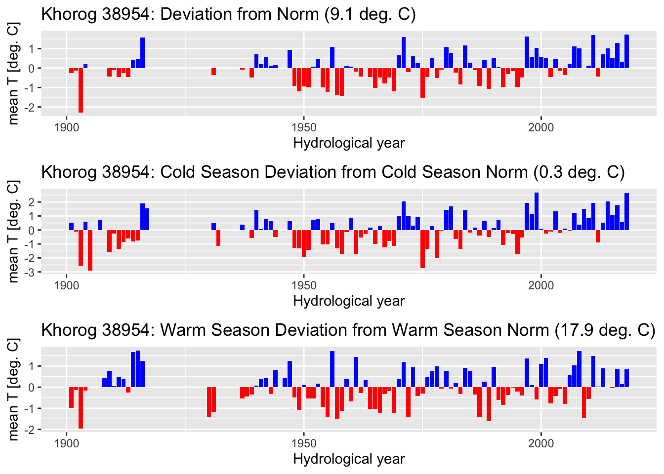
Figure 3.9: Annual devations from the norm of the mean temperature for the Khorog station 38954 record are shown for the entire hydrological year and for the corresponding cold and warm seasons. Note that the entire data record is taken into account here from the start of the 20th century.
The data was kindly provided by the Tajik Hydrometeorological Agency.↩︎