6.6 Model Calibration and Validation
6.6.1 Basic Principles
The large number of parameters of the HBV model can be adjusted within reasonable ranges to make the simulated river discharge more similar to the measured discharge. This process is sometimes called history matching because past measurements are used to adapt the model parameters. The following two exercises are important for understanding hydrological models. They are relevant whether you work as a modeler or as a decision maker. Try to first come up with a few own ideas and then study the solutions carefully. They will be discussed in the lectures in more detail.
E4.7
Model calibration - Common difficulties
Discuss with your colleague(s): What are typical difficulties inherent to the calibration of common semi-distributed (or fully distributed) hydrological models?
Hint: Compare the number of parameters of the HBV model to the number of model states.
E4.8
Model calibration - Strategies to handle the difficulties
Discuss with your colleague(s): Based on the list of common difficulties in the solution of exercise 5, think about possible strategies to address these challenges.
Hint: A modeler proverb says "as simple as possible but as complex as necessary".
6.6.1.1 Calibration vs. validation
As you have learned, semi- and fully distributed hydrological models are typically not well defined, i.e. you will find multiple sets of parameter combinations which will all yield reasonable model performance. An important strategy to gain confidence into a model is to split your time series into a calibration period and a validation period. During calibration, you adjust the model parameters to get a satisfying fit with the measured discharge. During the validation period you check how the calibrated model compares to discharge data that it hasn’t seen before, i.e. you judge the ability of the model to handle potentially different model input than it has seen during calibration. For example, if you have 30 years of discharge time series available you can use the first 10 years for model calibration (i.e. you run the model calibration procedure only over the first 10 years of the time series) and use the last 20 years for model validation. A good model should perform satisfactorily not only during calibration but also during validation.
In hydrology, it is recommended to do cross-validation, i.e. to calibrate and validate a model with several combinations of calibration and validation periods and to summarize the overall model performance.
Interested readers are refered to the literature for a more thorough discussion of the topic. For example, Bergstroem (Bergström 1991) gives a thorough discussion of model calibration and validation based on the HBV model which is still valid today.
6.6.1.2 Performance indicators
Model performance can be expressed in different ways. Some indicators are better suited to calibrate high flows (e.g. root mean squared error) and some are better suited to calibrate low flows (e.g. Nash coefficient for logarithm values). Others evaluate the models ability to reproduce the exceedance of a given discharge which is especially important for flood modelling. The calibration result depends on the choice of the performance indicators. For the automated calibration in RS Minerve, the user can choose a combination of several performance indicators. Care has to be taken to choose them according to the models goal.
E4.9
Model performance indicators
The RS Minerve technical manual summarizes the most important performance indicators typically used in hydrological modelling. For the more ambitious modellers, the manual includes references to the literature.
Read Chapter 3 of the technical manual.
6.6.2 Practical Steps
6.6.2.1 Manual calibration of synthetic discharge
The following section describes the steps for manual model calibration. We use the example of the Nauvalisoy river catchment and calibrate it with synthetic discharge measurements to deepen our understanding of the HBV model. For the synthetic discharge measurements it is theoretically possible to find a perfect match between simulated and measured data which is typically not the case for real measurements.
Add a comparator and a source object to your Nauvalisoy model and load river discharge measurements (filename), then run the model Here is a detailed step-by-step description of how to do this. With default parameters, the outcome of this step should look like Figure 6.12. Should your result differ significantly from the one shown here, compare the parameters of the HBV mode to the ones in the file ./data/SyrDarya/Chirchiq/RSMinerve/nauvalisoy_PAR_precalibration.txt. You can import the parameter set to RS Minerve via Import P in the model properties toolbar.
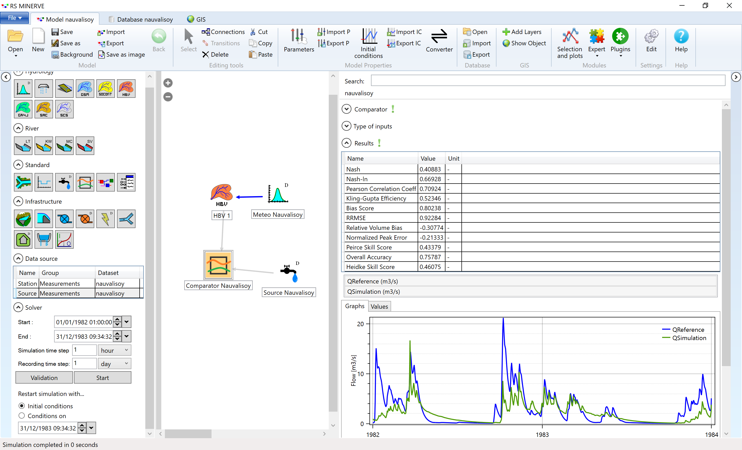
Figure 6.12: The simulated discharge (green) differs from the reference discharge (blue) before model calibration.
E4.10
RS Minerve - Manual calibration of synthetic discharge
1. Try to calibrate the model. Start with the parameters of the snow function and then proceed downwards through the compartments of the HBV model. Try to figure out which parameters influence the timing of the discharge peak, which the height of the peak and which the form of the recession curve.
2. Look at the variables of the HBV model during calibration (e.g. snow water equivalent, soil moisture, etc.).
Hint: This is an iterative process, give yourself some time for this task before you go peaking in the results.
The parameters of the calibrated model are linked here. Inspiration for this exercise from Prof. Jan Seibert and colleagues.
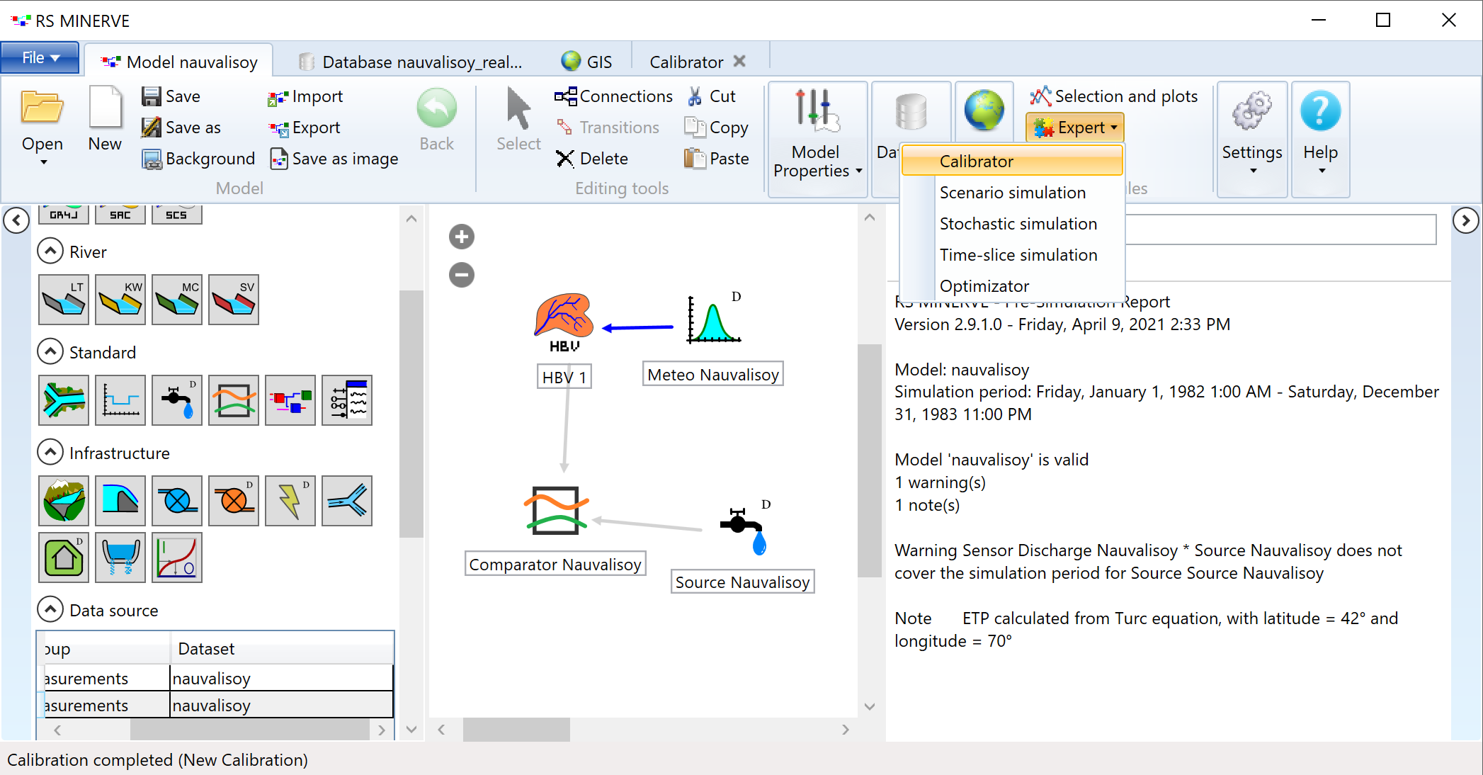
Figure 6.13: Open the calibration tab in RS Minerve.
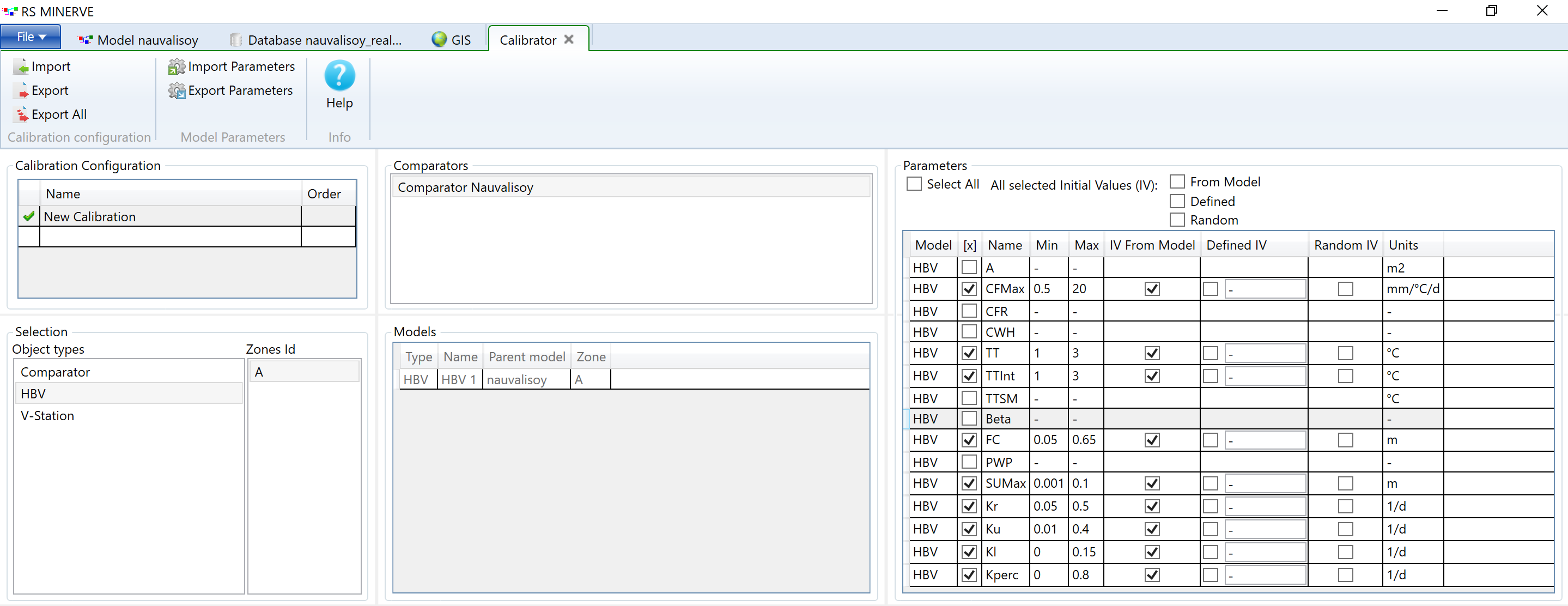
Figure 6.14: Open the calibration tab in RS Minerve.
You will have to choose performance indicators which will be combined in the objective function.
E4.11
RS Minerve - Automated calibration
Choose one or several performance indicators and run the automated calibration. The automated calibration may take a few minutes (expect around 3000 model iterations). Compare the parameters found with the automated calibration to the ones that were used for the generation of the synthetic discharge values (in solutions of the manual calibration example). Discuss the differences. Where were you surprised? Which parameters could be identified and which not?
Change the combination and weights of the performance indicators and redo the automated calibration. Note how the calibration result changes.
You have seen in the exercise above that is not so easy to find the true parameter set of a basin. Let’s get a better understanding of the model parameters. Choose 1-3 parameters for which you will do a sensitivity analysis.
E4.12
RS Minerve - Manual sensitivity analysis
Discuss with your colleague(s) in which way you expect the model outcomes to change when you modify your chosen parameters before you run the model.
Make notes of the changes in parameters and the changes in the model outcomes.
The sensitivity analysis can be automated in RS Minerve. Make sure to have the calibrated parameter set loaded (via import P in the Model Properties toolbar). Open the tab for stochastic simulations in the Module toolbar (see Figure 6.15).
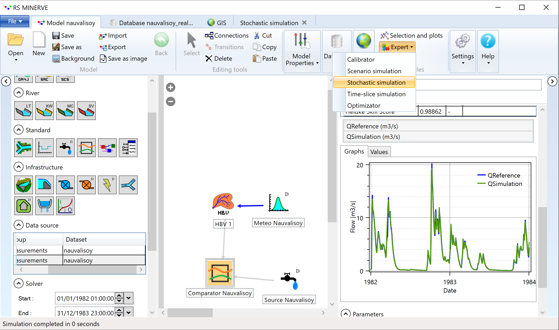
Figure 6.15: Open the stochastic simulation tab in RS Minerve.
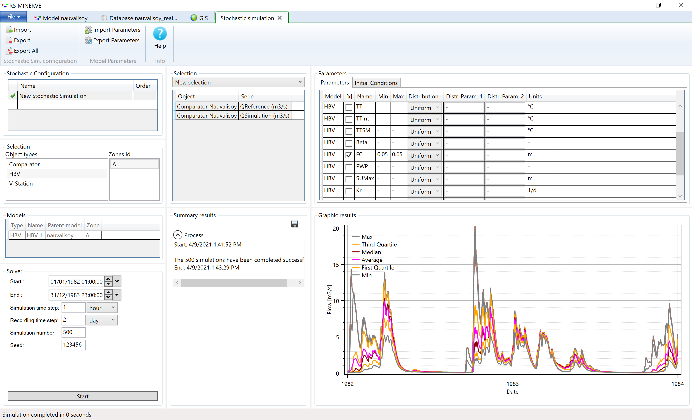
Figure 6.16: Open the stochastic simulation tab in RS Minerve.
E4.13
RS Minerve - Automated sensitivity analysis
Perform an automated sensitivity analysis for the same parameters you chose in the previous exercise (manual sensitivity analysis).
Compare the outcome of the manual sensitivity analysis.
Bonus task: Choose a sensitive model parameter and evaluate the sensitivity of the stochastic simulation with regard to the number of simulations or the seed. (The seed is used in the random number generator. It makes the stochastic simulation reproducible.)
Figure 6.17 shows the resulting discharge time series in the comparator object.
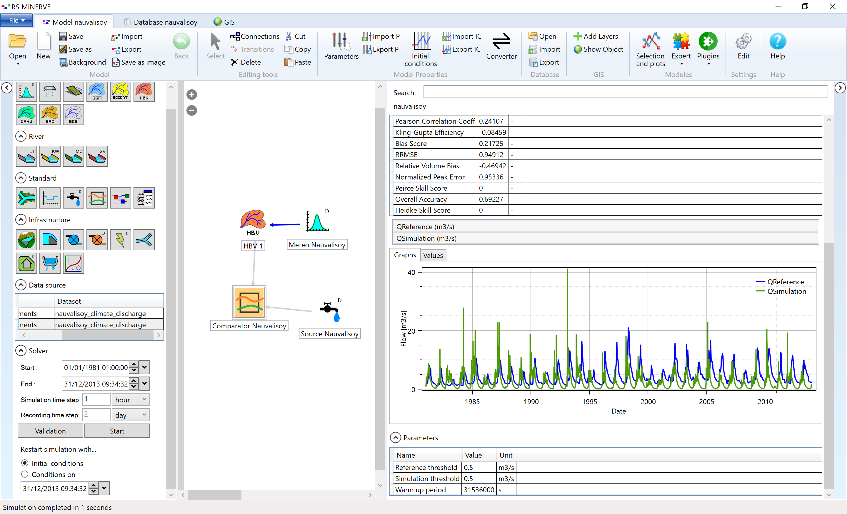
Figure 6.17: Simulated and measured discahrge at the outlet of the Nauvalisoy catchment.
The simulated discharge peak arrives several months before the observed discharge peak. You may invest 10 minutes to try it out but by merely adjusting the parameters of our HBV model, we will not be able to shift the simulated discharge time series sufficiently to reproduce the measured discharge. We are facing a conceptual model error which we have to identify and eliminate.
Figure 6.18 shows the relationship between elevation and temperature of the 4 meteo stations in the Gunt river catchment. The elevation dependence of temperature is highly important for snow-melt driven river catchments.
## MeteoStation locations and elevation
meteoStations <- # just put everything in a regular dataframe
  tibble(code = c(38953, 38954, 38956, 38950),
         masl  = c(3746, 2075, 3438, 2566))

# Load Gunt data
data <- read_rds('./data/AmuDarya/Gunt/StationData/gunt_data_cleaned.Rds') %>%
  dplyr::filter(str_detect(type, "T")) %>%  # Filter for data types that contain T
  mutate(code = as.numeric(code)) %>%  # Cast code column to numeric
  left_join(meteoStations)  # Add the station altitude to the data

# Plotting the dataframe
data %>%
#   dplyr::filter(!str_detect(type, "meanmax"),
#                 !str_detect(type, "meanmin")) %>%
  dplyr::filter(str_detect(type, "mean\\(T\\)")) %>%
  dplyr::mutate(Variable = type) %>%
  group_by(code, Variable) %>%
  summarize(norm = mean(norm, na.rm = TRUE),
            masl = first(masl)) %>%
  ggplot(aes(norm, masl)) +  #, colour = Variable)) +
  geom_smooth(method = "lm", alpha = 0, colour = "gray") +
  geom_point() +
  labs(y = "Altitude [masl]", x = "T [deg C]") +
  theme_bw()
Figure 6.18: Elevation dependence of mean temperature at the four meteo stations in the Gunt river catchment. The temperature decrease is a little below 1 degree K per 100 m of altitude gain.
At temperatures below approximately 0 degrees C, precipitation falls as snow and remains stored as snow in the catchment until temperatures above 0 degrees C melt the snow and produce runoff. Especially for snow driven catchments, it is important to take the elevation dependence of temperature into account. In RS Minerve, this can be done by dividing the catchment into several sub-catchments of similar altitude (i.e. elevation bands) and to define temperature (and precipitation) inputs for these sub-catchments. This is a spatial refinement of the model which allows us to better represent the snow storage and melting processes in the catchment. A description of how to obtain the elevation bands is given in the Chapter on the preparation of geospatial data.
6.6.2.2 Spatial refinement of the model
** TODO: Nauvalisoy elevation bands at higher resolution, ask tobi how involved the exctraction of the era5 bias corrected data for the elevation bands is **