5.2 Geospatial Data
This Section follows the steps shown in Figure 5.1 and explains in a hands-on manner how to arrive at and process the required geospatial data for later inclusion in the hydrological-hydraulic model RS Minerve Links to detailed descriptions of the individual tasks allow even beginners of QGIS to follow the procedure. The requirements for GIS layers for import in RS Minerve are summarized in Figure 5.10.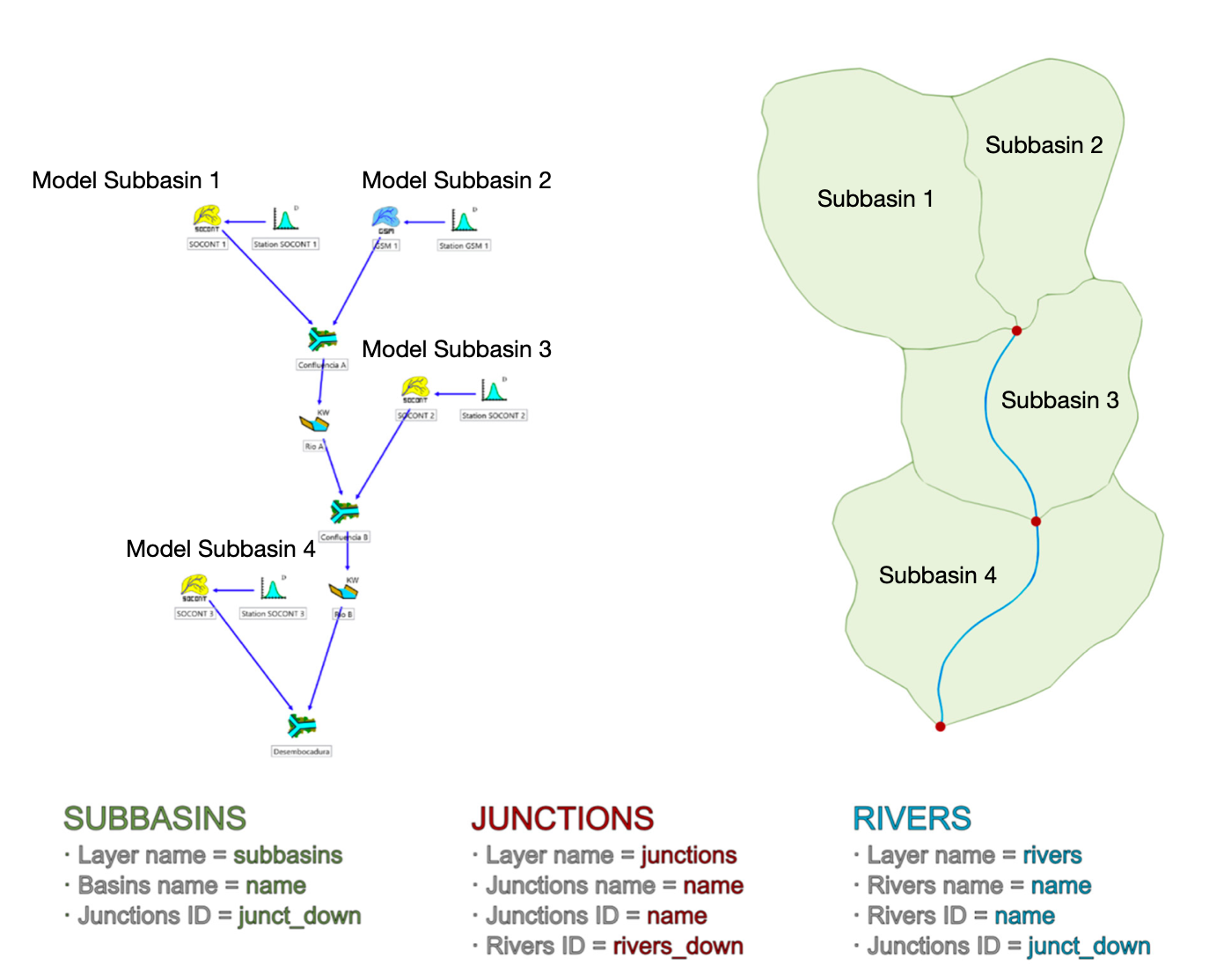
Figure 5.10: Required GIS input files for RS Minerve. See corresponding user manual for more information.
RS Minerve connects the sub-basins to junctions. River stretches run from upstream junction to downstream junction. The names of the junctions need to be consistent throughout the GIS layers.
In this chapter we will demonstrate how to derive the GIS layers for the Nauvalisoy river catchment. The Nauvalisoy is a small tributary to the Chirchiq river (see Figure 3.10 in the case studies). It does not include channel routing.
E5.1
Prepare GIS layers
Go through the steps in this Chapter to generate yourselves the GIS layers of your sample catchment for import into RS Minerve.
5.2.1 Prerequisites
- QGIS must be installed (QGIS installation guide).
- Coordinates of a discharge gauge in your sample catchment are available in the learningFiles directory.
- A digital elevation model (DEM) for your sample catchment is available in the learningFiles directory. A description of how to obtain a free SRTM DEM is given below.
5.2.2 Setting up QGIS
- Open and save a new QGIS project (How to for absolute beginners).
- Make sure that the projects projection is in UTM (How to change the projection of a project).
- Check if the required plugins (qProf or profile tool) are installed (How to install and activate a plugin).
- The optional plugins are: SRTM plugin (requires a login to USGS Earth Explorer How to register).
- The optional plugins are: SRTM plugin (requires a login to USGS Earth Explorer How to register).
- Note that SAGA GIS and GRASS GIS must be installed and correctly configured in QGIS (which is typically the case for default installations of long-term support versions of QGIS).
5.2.3 Load DEM
You will find a DEM raster layer in the ./learningFiles directory of your sample catchment ready to start. Load the DEM into your QGIS project and save the project (how to). For the hydrological analysis, the DEM needs to be in UTM projection. Look up the projection of your DEM layer and re-project to UTM if necessary (how to).
The description of how to obtain the DEM is given here: We use the SRTM 1 arc-second global DEM (Data description). The DEM tiles are downloaded directly in QGIS3 (SRTM plugin, How to) or via the USGS Earth Explorer (How to) and merged to a single GIS layer (How to). In any case you will need to register for an Earth Explorer account How to register.
Typically, geospatial data from open sources is stored in the standard projection WGS84 (EPSG:4326). The WGS84 is in degrees, minutes and seconds but for hydrological analysis it is more convenient to have spatial layers in the UTM projection. Look up in which UTM Zone your catchmen lies and re-project to that Zone. For the example of the Chirchiq basin, the UTM zone is 42N, i.e. EPSG:32642.
5.2.4 Catchment delineation
For this workshop, shapefiles for the sample watersheds you will model are already available in the shared dropbox folder with the data for case studies which you should have already downloaded. Load the shape file of your sample catchment into QGIS (how to add a vector layer).
In case you’d like to learn how to delineate your own watershed, follow the tutorial below. The steps are also described in this tutorial on youtube
Projection of DEM
Verify that the DEM is in UTM coordinates and re-project it if necessary (how to).
Fill the sinks of the DEM
To derive the the catchment area upstream of a discharge gauge, the DEM is traced upstream until elevation values do not increase any more, i.e. until the boundary of the watershed is reached. The SRTM DEM contains the rounded average elevation in each cell of about 25-30m resoluition. Due to the averaging and rounding it may happen, that in a SRTM DEM, an upstream river cell contains lower elevations than the downstream river cell. If the catchment delineation algorithm reaches such a situation, it stops, thinking it has reached the boundary of the watershed. To avoid this, cells that form local depressions should be filled to form a river bed which is continuously increasing in elevation until it reaches the watershed boundary. The SAGA algorithm to do this is called Fill sinks.
Fill the sinks of your DEM and store the processed raster file (how to in detail).
Upslope area
Determine the area up-slope of your river discharge gauge by running the algorithm Upslope Area in QGIS (detailed instructions). The UTM coordinates of the Nauvalisoy discharge gauge are given in the riversCentralAsia package:
dplyr::filter(ChirchikRiverBasin, river=="Nauvalisoy") %>%
  dplyr::summarize(`Station code` = dplyr::first(code),
                   `Station name` = dplyr::first(station),
                   `River name` = dplyr::first(river),
                   Longitude = dplyr::first(lon_UTM42),
                   Latitude = dplyr::first(lat_UTM42))
## # A tibble: 1 x 5
## `Station code` `Station name` `River name` Longitude Latitude
## <chr> <chr> <chr> <dbl> <dbl>
## 1 16298 Sidzhak Nauvalisoy 589674 4618690The Upslope Area function will return a raster file of your catchment area. Convert it to a polygon and save the resulting shape (how to convert raster to polygon).
Now you have a DEM and a watershed boundary ready. The steps to generate the GIS layers for import in RS Minerve are numerous. We have generated the input files for the sample catchments for you. In case you wish to reproduce the steps you can follow the description below.
5.2.5 Run through the process model
A process model is available that generates the raw GIS layers for RS Minerve. Navigate to Processing and open the Graphical Modeller…. The Model Designer window opens. Open the model downloaded from here: ./model/Basin_Preparation_QGIS.model3 (5.11).
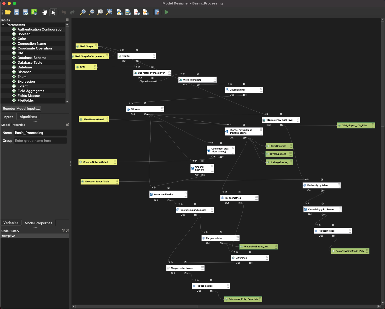
Figure 5.11: The process of deriving the GIS layers for RS Minerve is simplified through the process model.
Prior to running the model, read through the following brief notes.
Input files
- A shape file of the basin outline in UTM 42 N. A shape file is provided in the Case Study Packs folder on Dropbox that you should have already downloaded. Here is a description of how to derive the basin outline if you need to do so for a future project.
- The extent of the DEM needs to be larger than the boundaries of your catchment. You can use the raw SRTM DEM projected to UTM42N that is provided in the Case Study Packs folder on Dropbox. If you want to download the DEM yourself you find a description of how to do so here.
Model output
Besides the 3 layers required for RS Minerve (compare Figure 5.10):
- Basins: BasinElevationBands_Poly_fixed
- Rivers: RiverChannels
- Junctions: RiverJunctions
The model produces a number of additional output files which can be used for verifying the parameterisation which is described in more detail in the next section.
5.2.5.1 Parameterization of the model
- BasinShapeBuffer_meters is a buffer around the basin outline to which the DEM is cut. The DEM needs to be slightly larger than the shape line. The default value of 1000 m is sufficient, 500 m work as well.
- The Channel Network Cutoff Value is a parameter required for the partitioning of the catchment into sub-catchments. Values between 2e8 and 5e8 have been found to work well for smaller and medium sized catchments. The model is sensitive to this parameter and might throw an error if the cutoff value is not appropriate.
- The Elevation Bands Table holds the altitude boundaries and class IDs for the elevation bands in the catchment. After a first test run, edit according to your needs. Elevation bands of 200 m intervals are typically chosen to sufficiently refine the elevation dependent snow melt. For your case study you may use an interval for the elevation bands between 500 m for smaller catchments and 1000 m for larger catchments.
- River Network Level is a parameters for the resolution of the river network. Values of 7 and 8 have shown good results for smaller and medium sized catchments (Figure 5.12).
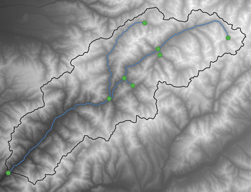
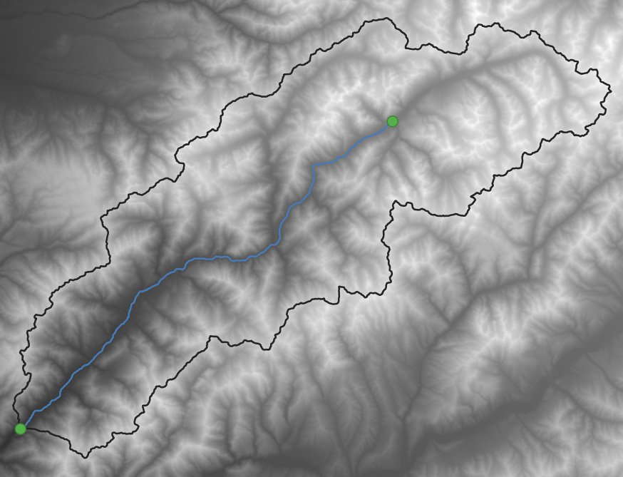
Figure 5.12: Comparison of River Network Level = 7 (left) and River Network Level = 8 (rigth) for the example of the Pskem river catchment.
The model is sensitive to these parameters. Play around with them until you are satisfied with the resulting GIS layers.
Trouble shooting
If you get an error message running Fix geometries that POLYGONS.shp was not found, try reducing the Channel Network Cutoff Value by 50-70%. You can still inspect the other layers and change other parameters as well.
- Make sure that all input layers are projected to UTM 42 N.
- Run the model through once, inspect the output and play with the input parameters:
- Min and Max elevations on the smoothed DEM and the shape, number and spacing of elevation bands (edit the table for the elevation bands accordingly),
- Location and shape of river reaches and the location of junctions (vary the threshold).
- Min and Max elevations on the smoothed DEM and the shape, number and spacing of elevation bands (edit the table for the elevation bands accordingly),
For the example of the small Nauvalisoy river basin, the parameterization is given in Figure 5.13.
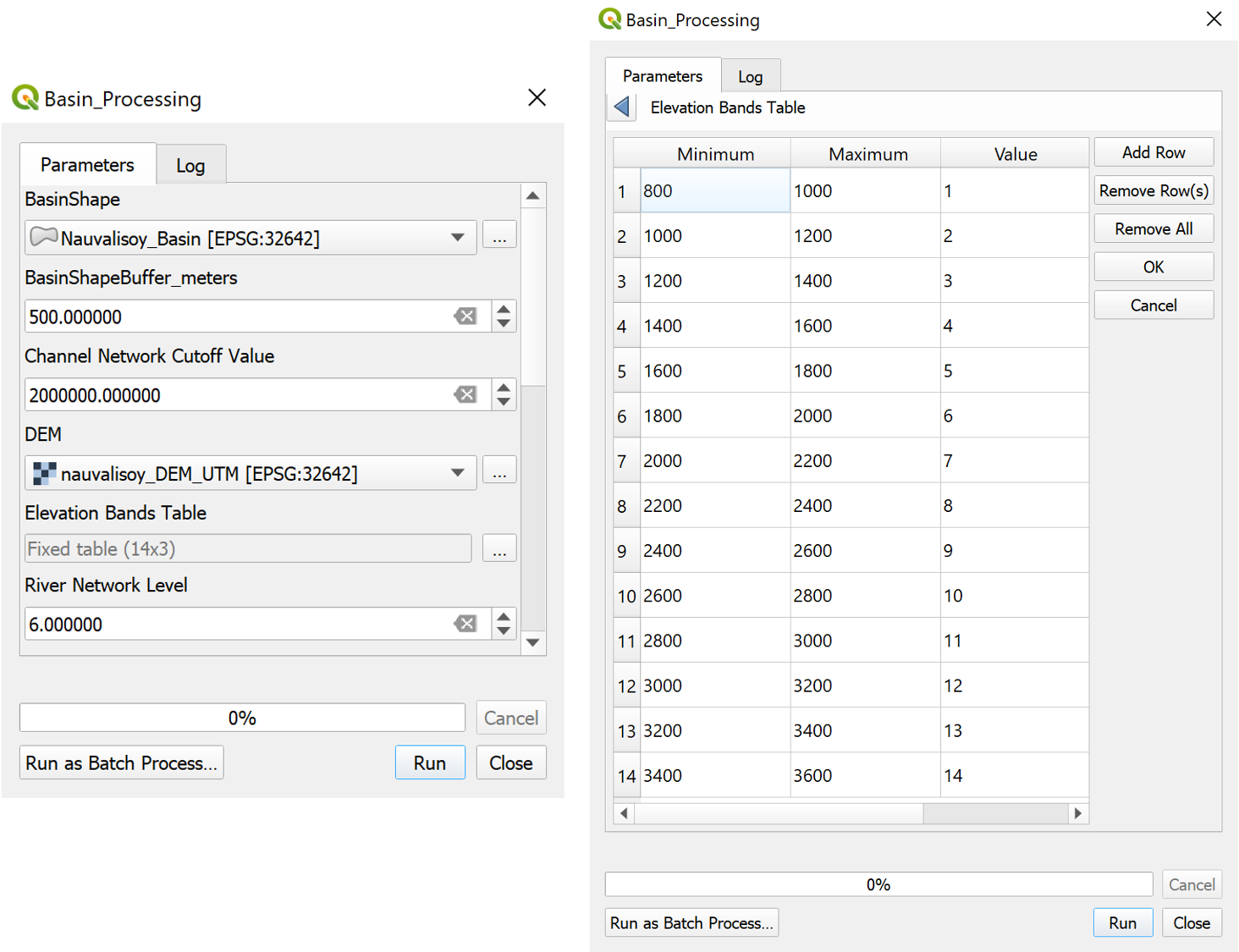
Figure 5.13: Parameters for the basin processing model chain for the Nauvalisoy catchment.
Resulting layers of the QGIS model chain
The Output layers of the QGIS model process are shown in Figure 5.14.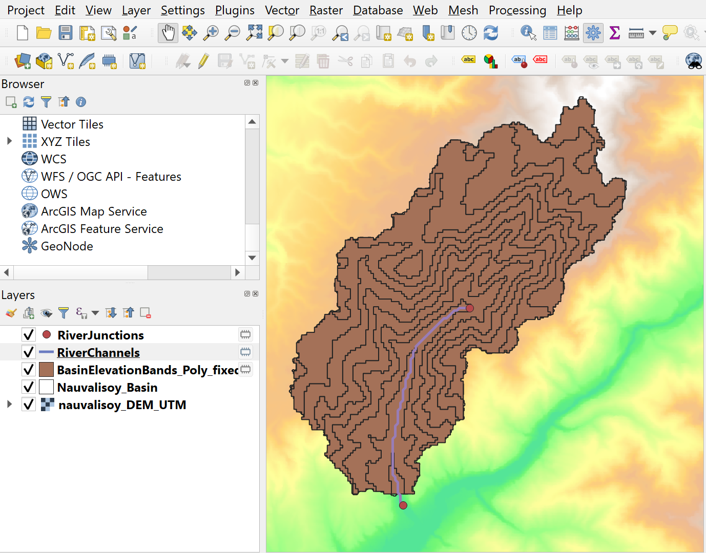
Figure 5.14: Raw output of the QGIS model chain to derive the GIS layers for import into RS Minerve.
Let’s inspect the GIS layers and determine which edits are still necessary.
5.2.6 Manually edit the GIS layers for import in RS MINERVE
The basin layer
Verify that the elevation bands are numbered in the correct order. You can do this for example by opening the attribute table, sorting the IDs in ascending order and click through the layers. The selected feature is highlighted in yellow in the map panel and should move along the as you select the next row (see Figure 5.15).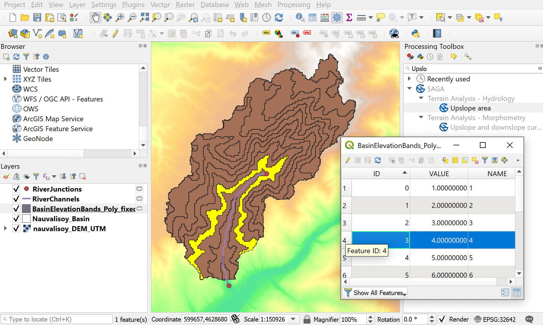
Figure 5.15: Verify that the elevation bands are in the correcto order.
Also, there should only be one row per ID in the attribute table. If the QGIS model process has run through correctly, this should be the case. Each of the sub-basins in the basin layer will be translated to a hydrological model in RS Minerve.
RS Minerve requires the specification of the downstream junction for each sub-basin (compare Figure 5.10). Toggle the edit mode by pressing the pen icon in the upper left corner of the attribut table window. Press the New Field icon (Figure 5.16)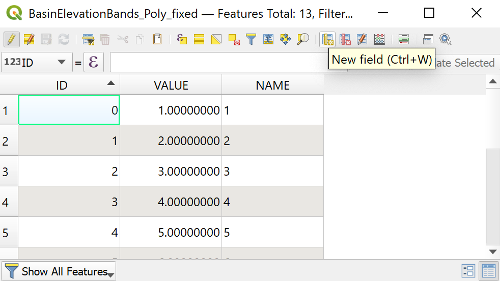
Figure 5.16: Press Add New Field in the toolbar of the attribute table.
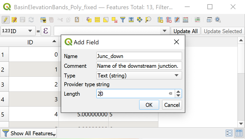
Figure 5.17: Enter the attributes of the new field.
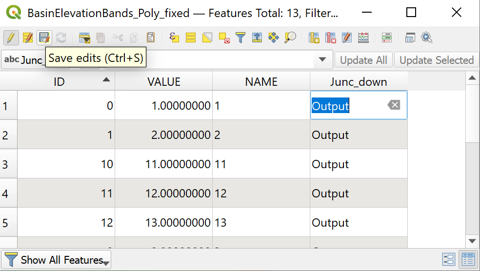
Figure 5.18: Edit the junction names and save your changes.
Save the edits and un-toggle the edit mode by pressing on the pen icon. You can close the attribute window. If the layer is still temporary, you can store save it to your computer (how to save a temporary layer).
The junctions layer
The output of the QGIS model process shows two junctions (see Figure 5.14). We only need to keep the junction at the outlet. Select the RiverJunctions layer in the Layers panel open the attribute table. There select the column with ths spring node, toggle the edit mode and delete the node by pressing on the icon with the red bin. The outlet node is already called Outlet so we do not need to change this name, it is already consistent with the basins layer. Save your edits and un-toggle the edit mode. Close the attribute table and save the junctions layer.
An alternative way to edit the junctions layer, especially if you have larger and more complicate catchments, is via the graphical editor. A detailed description of how to do this is given in the Appendix
The river layer
Although we will not implement river routing in the hydrological model for the Nauvalisoy basin, RS Minerve requires a GIS layer for the river. Edit the RiverChannels layer as follows in the attribute table: Press the Delete fields button (Figure 5.19).
Figure 5.19: The delete fields button in the attribute table toolbar.
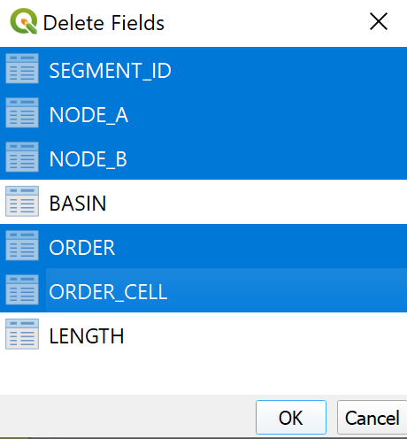
Figure 5.20: Select the fields of the attribute table to delete.
Add a field for the downstream junction and enter Outlet you can proceed in the same way as described above for editing the basin layer. Save the river channels layer.
If you have larger catchment with a more complex structure to edit you may be interested in a detailed description of the graphical editing of GIS layers in the Appendix. The example shows editing of a junction layer but you may proceed in the same manner for editing the rivers layer.
The layers are now ready for import into RS Minerve. This will be described in Chapter 6.4.