5.3 Climate Reanalysis Data

Information about the spatio-temporal distribution of precipitation (P) and temperature (T) is vital for water balance studies, including for modeling. Poorly gauged basins do not have dense enough ground-based monitoring network that would allow to obtain reliable meteorological fields that can be used to drive hydrological models. Station data are especially poor in complex and remote mountain catchments in developing and transition countries. The Central Asian river basins are examples of such basins. Global reanalysis data can help to cover these existing gaps. In this Chapter, we show how this can be achieved.

We use ERA5 global reanalysis data to obtain temperature at 2 meters above ground and total precipitation fields on an hourly base from 1981-01-01 through 2020-12-31. ERA5 data comes with a 30km grid cell size resolution and is thus quite course. This is relevant for complex mountain terrains which feature highly variable climate over very short distances, sometimes from one valley to the next. To address this problem, a bias correct version of the monthly CHELSA high resolution climatology product is used to arrive at high resolution hourly climatology fields (the CHELSA dataset is described in (Karger et al. 2017) and the bias correction of it in (Beck et al. 2020b). Like this, high-resolution hourly data from 1981-01-01 through 2013-12-31, i.e. the period for which the CHELSA dataset is available, could be derived. These data are then used for model calibration and validation and for the computation of the reference hydro-climatological situation from 1981 through 2013. More details can be found in Chapter 6.

The analysis present here is for the Gunt river catchment. The approach and methods we have developed are universally applicable for other catchments.

5.3.1 CHELSA V1.2.1 Data and Bias Correction

The CHELSA V1.2.1 data covers the period 1981-01-01 until 2013-12-31. This period is considered to be the base climate period where 1981-01-01 until 1993-12-31 will be used as the parameter calibration period for the hydrological model. The model validation period is from 1994-01-01 until 2013-12-31. This period will constitute the baseline period in relation to which climatic changes in the mid 21st as well as end of 21st century will be assessed.

Mean monthly temperature and total monthly precipitation between 1981-01-01 and 2013-01-01 can be accessed and downloaded for the Central Asia domain from the following online repository⁷. Mean monthly temperatures are stored in the ./t2m/ folder and precipitation in the ./pr/ folder there.

Note that the Central Asia domain is defined as test

aoi_CentralAsia_LatLon <- extent(c(65,80.05,35.95,44.05)) # this is a raster::extent() object. For more information, type ?extent into the console.

The CHELSA data are downscaled ERA-INTERIM model outputs for temperature and precipitation with a resolution of 30 arc seconds (Karger et al. 2017). Temperature fields are statistically downscaled ERA-INTERIM temperatures whereas for precipitation downscaling, several orographic predictors are taken into account, including for example wind fields, valley exposition, height of the atmospheric boundary layer, etc.

Because of its highly resolved climatologies, the CHELSA data has been shown to be particularly useful for studies in regions with complex topography. However, it has also been shown that the original CHELSA precipitation data is underestimating high mountain precipitation. This can be explained by the phenomenon of snow undercatch which explains measured precipitation deficits by sublimation and blowing snow transport at high altitude meteorological stations.

An example of this is shown in Figure 5.21 for high elevation gauges in Spain. In a recent intercomparison project carried out in Spain, it has been shown that undercatch poses significant problems in accurately measuring solid precipitation (Buisán et al. 2017) in mountainous regions. Both, ERA-INTERIM and CHELSA themselves assimilate station data in their models and hence are affected by these erroneous measurements.

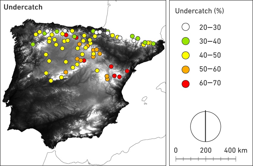
Figure 5.21: Measured snow undercatch values in high-mountain stations in Spain. The values were determined within the World Meteorological Organization Solid Precipitation Intercomparison Experiment (WMO-SPICE). See text for more information and reference.

Beck et al. (2020a) has recognized this and released monthly correction factors for the CHELSA data (see Figure 5.22).

Figure 5.22: Figure from (Beck et al. 2020a), Supplementary Material. Plate d): Best estimate of global bias correction factors. Plate e): Lower bound estimate of global bias correction factors. Plate f): Upper bound of global bias correction factors. As is clearly visible, bias correction factors in high-mountain Asia, including the parts of Central Asia are significant.

The bias corrected CHELSA precipitation (tp) raster data is available via this Dropbox link. Using these temperature as well bias-corrected precipitation data, we can easily compute and display the monthly norm climatology fields over the Central Asia domain⁸. Here, we just load them and visualize the mean monthly patterns for a consistency check.

t2m_meanMonthlyClimate_CHELSA <- 
  raster::brick('./data/CentralAsiaDomain/CHELSA_V1.2.1/t2m_climatology/t2m_climatology_CA.tif')

names(t2m_meanMonthlyClimate_CHELSA) <- month.abb
t2m_meanMonthlyClimate_CHELSA <- t2m_meanMonthlyClimate_CHELSA / 10 - 273.15 # now, the CHELSA data is in deg. C

temperature_colors <- brewer.pal(9, "RdYlBu") %>% colorRampPalette()

gplot(t2m_meanMonthlyClimate_CHELSA) + 
  geom_tile(aes(fill = value)) +
  facet_wrap(~ variable) +
  scale_fill_gradientn(colours = rev(temperature_colors(5))) +
  coord_equal() +
  guides(fill=guide_colorbar(title='T [deg. C.]'))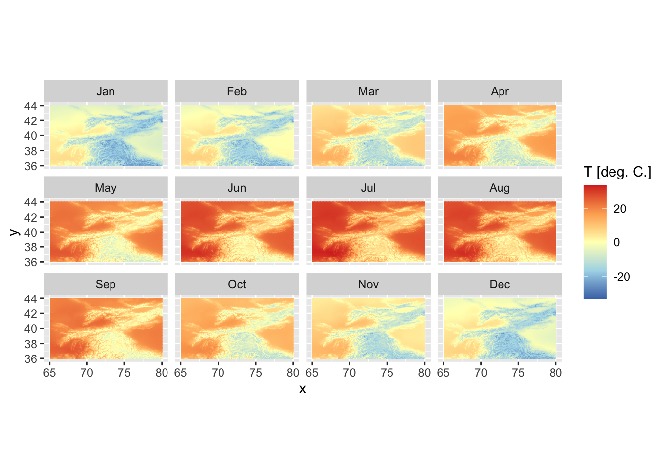 

Figure 5.23: CHELSA v1.2.1 mean monthly temperature climatology is shown.

In a similar way, the bias corrected precipitation climatology can be plotted. Figure 5.24 nicely shows the main precipitation months of the key mountain ranges in the region. The Figure shows that March and April are normally the main precipitation months.

# Load file
pbcorr_pr_meanMonthlyClimate_CHELSA <- 
  raster::brick('./data/CentralAsiaDomain/CHELSA_V1.2.1/pr_climatology/pr_climatology_CA.nc')
# Layer names
names(pbcorr_pr_meanMonthlyClimate_CHELSA) <- month.abb
# Color palette
precipitation_colors <- brewer.pal(9, "YlGnBu") %>% colorRampPalette()
# Plot
gplot(pbcorr_pr_meanMonthlyClimate_CHELSA) + 
  geom_tile(aes(fill = value)) +
  facet_wrap(~ variable) +
  scale_fill_gradientn(colours = precipitation_colors(500)) +
  coord_equal() +
  guides(fill=guide_colorbar(title='P [mm/yr]'))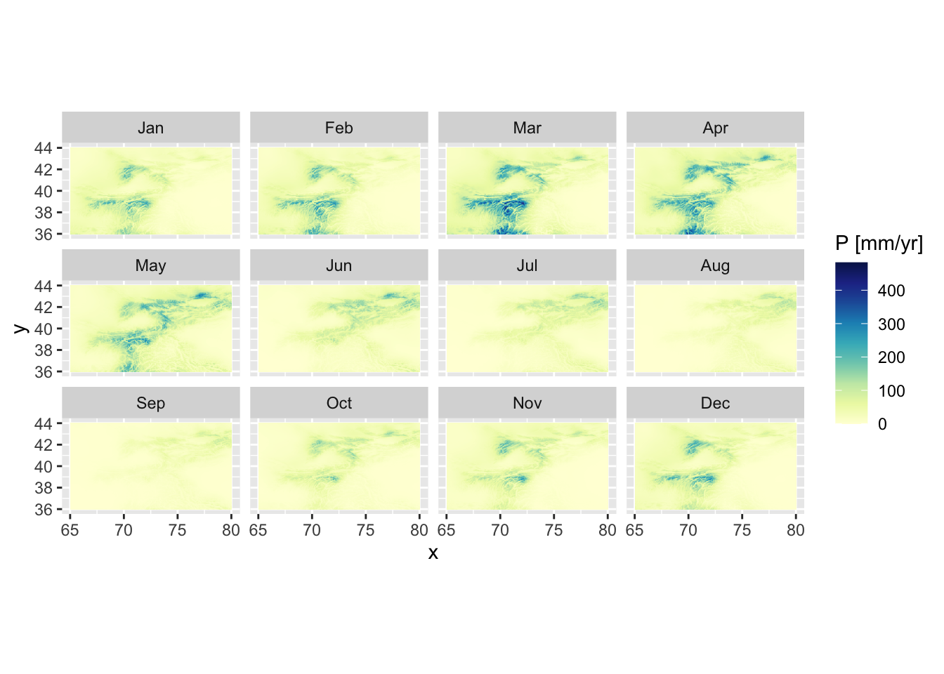 

Figure 5.24: CHELSA v1.2.1 mean monthly precipitation climatology is shown.

How can the quality of the CHELSA data in the complex Central Asia domain be assessed? We explore this question the validity of the CHELSA dataset to be able to adequately represent the high-mountain climate in the Pamirs. The key questions here to be answered are

• does the magnitude of the precipitation yield physically meaningful results, and

• does the climatology adequately reproduce the seasonal cycle observed one at the stations?

Let us address the first question investigating bias corrected precipitation values and comparing these discharge for the Gunt river basin. If \(P >Q\) where \(P\) is the long-term mean precipitation and \(Q\) is the long-term mean discharge, we can confidently say that the bias corrected CHELSA precipitation product is meaningful from a water balance perspective (see also Chapter 4 for more information).

# Load catchment shp
gunt_Shapefile <- st_read('./data/AmuDarya/Gunt/GeospatialData/Gunt_Basin_poly.shp',quiet = TRUE)
gunt_Shapefile <- gunt_Shapefile %>% subset(fid==2)
gunt_Shapefile_LatLon <- st_transform(gunt_Shapefile,crs = st_crs(4326))
areaGunt <- gunt_Shapefile %>% st_area() %>% as.numeric()

# Areas of Interest
aoi_CentralAsia_LatLon <- extent(c(65,80.05,35.95,44.05)) # in lat/lon
aoi_Basin_LatLon <- gunt_Shapefile_LatLon %>% extent() # GUNT
aoi_Basin_UTM <- gunt_Shapefile %>% extent() # GUNT, in UTM

fLoc <- './data/AmuDarya/Gunt/ReanalysisData/tp_bcorr_NORM_CHELSA_Gunt.nc'
chelsaP_GUNT_corr_raster <- brick(fLoc, varname="corr_P_annual")

chelsaP_GUNT_corr__spdf <- as(chelsaP_GUNT_corr_raster, "SpatialPixelsDataFrame")
chelsaP_GUNT_corr__df <- as.data.frame(chelsaP_GUNT_corr__spdf)
colnames(chelsaP_GUNT_corr__df) <- c("value", "x", "y")

# Plot the raster for inspection and analysis
ggplot() +
  geom_tile(data=chelsaP_GUNT_corr__df, aes(x=x, y=y, fill=value), alpha=0.8)+
  geom_sf(data=gunt_Shapefile,color="black",fill=NA) +
  scale_fill_gradientn(colours = precipitation_colors(5)) + 
  xlab("Longitude") + ylab("Latitude") + 
  guides(fill=guide_colorbar(title="P Norm [mm]")) + 
  ggtitle("Bias Corrected CHELSA v1.2.1 Norm Precipitation, Gunt River Basin")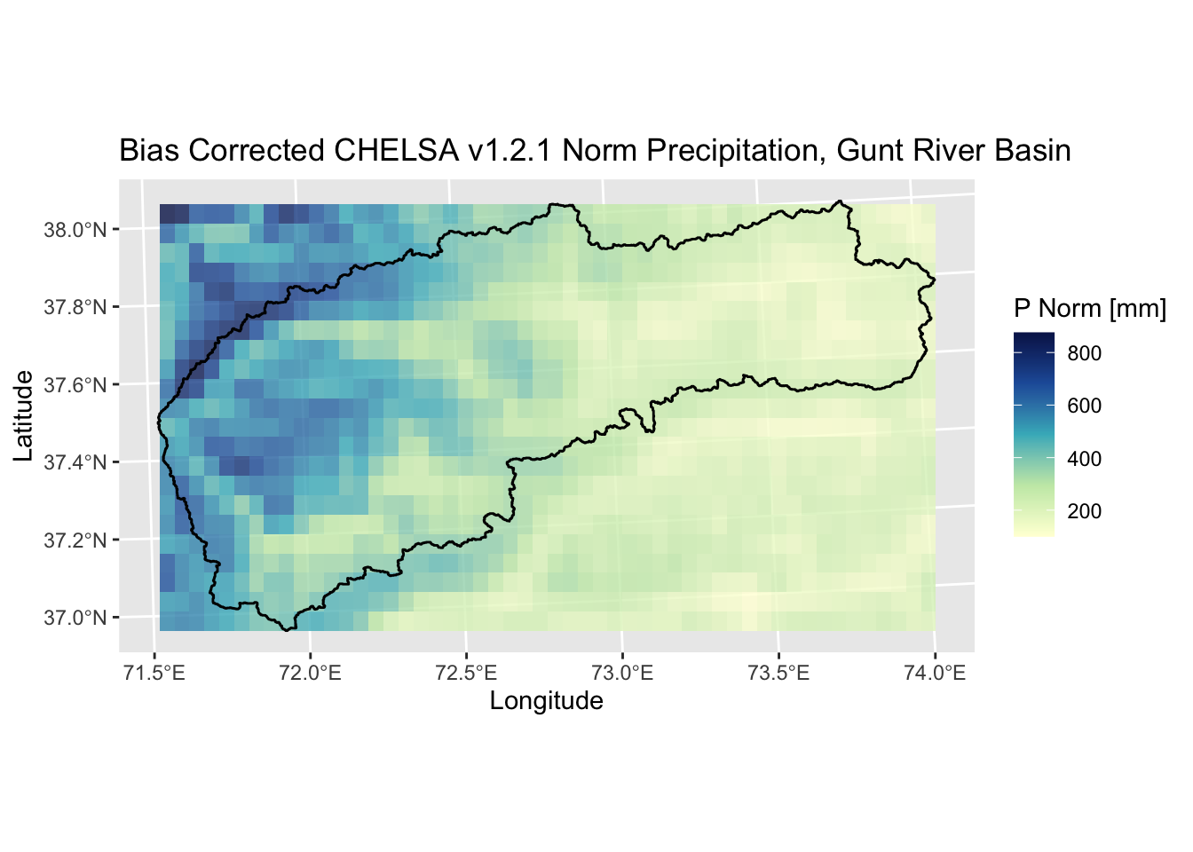

Figure 5.25: Long-term mean precipitation climatology of the Gunt river basin in the Pamir mountains. The catchment is delineated by the black polygon. The mean long-term precipitation in the catchment is 349 mm/year.

# Extract raster values inside basin polygon and convert to equivalent water height
rasterRes <- chelsaP_GUNT_corr_raster %>% res()
rasterCellArea <- rasterRes[1] * rasterRes[2] # in m^2
basin_P <- raster::extract(chelsaP_GUNT_corr_raster,gunt_Shapefile)[[1]] * rasterCellArea / 1000
basin_P <- basin_P %>% sum() / areaGunt * 1000 # now in mm
#print(paste0("The bias corrected CHELSA v.1.2 norm precipitation in Gunt River Basin is ", basin_P %>% round(0), ' mm'))

From the perspective of the water balance, the basin-wide long-term mean precipitation estimate passes the test since P (353 mm) > Q (234 mm) where the latter is the long-term discharge norm at the Khorog gauging station at the outlet of the basin (see also Chapter 3 for more information on Gunt river basin). The water balance components are also discussed in Chapter 4.

As an aside, the bias corrected precipitation climatology shows an interesting feature of the Gunt river basin (see Figure 5.25). Namely, there is a stark precipitation gradient between the western part of the basin where the bulk of the precipitation is observed and the hyper-arid Pamir plateau region to the east, where annual precipitation is around or below 200 mm.

What about the seasonality of the CHELSA product? Can it adequately reproduce the observed precipitation seasonality? If this would not be the case, we would have to reject the validity of the product and explore other high-resolution climatologies such as WorldClim V2 or CHPClim V1 (see (Beck et al. 2020c) for more information on these products). Lets explore again for Gunt river basin.

First, we load and prepare all the required station precipitation and geospatial data. Then, we compute the monthly norms of these data for the period 1981-01-01 through 2013-12-31.

# Get data (this time, we access the monthly norm data through the specification of the variable name, that we want to load, i.e. varname="corr_P_monthly") 
fLoc <- './data/AmuDarya/Gunt/ReanalysisData/tp_bcorr_monthly_CHELSA_Gunt.nc'
chelsaP_GUNT_monthly_corr_raster_proj <- brick(fLoc, varname="corr_P_monthly")

# Extract Gunt river basin cells and compute monthly totals
chelsa_monthly_norm_P <- extract(chelsaP_GUNT_monthly_corr_raster_proj,gunt_Shapefile)[[1]] * rasterCellArea / 1000
chelsa_monthly_norm_P <- (chelsa_monthly_norm_P %>% colSums() / areaGunt * 1000) %>% unname() # now in mm
chelsa_monthly_norm_P <- chelsa_monthly_norm_P %>% as_tibble() %>% rename(CHELSA_norm_P=value)

# Load Gunt Station Data record
fPath = './data/AmuDarya/Gunt/StationData/gunt_data_cleaned.Rds'
data <- read_rds(fPath)

# Prepare the station data precipitation record
P_38950 <- data %>% filter(type=="P" & code==38950) %>% dplyr::select(date,data) %>% rename(P_38950=data)
P_38953 <- data %>% filter(type=="P" & code==38953) %>% dplyr::select(date,data) %>% rename(P_38953=data)
P_38954 <- data %>% filter(type=="P" & code==38954) %>% dplyr::select(date,data) %>% rename(P_38954=data)
P_38956 <- data %>% filter(type=="P" & code==38956) %>% dplyr::select(date,data) %>% rename(P_38956=data)

P <- full_join(P_38950,P_38953,by="date")
P <- full_join(P,P_38954,by="date")
P <- full_join(P,P_38956,by="date")

# add a month identifier
P <- P %>% filter(date>=as.Date("1981-01-01") & date<=as.Date("2013-12-31")) %>% mutate(mon = month(date)) %>% 
  dplyr::select(-date)
P <- P %>% pivot_longer(-mon) %>% group_by(mon)

# Now, make a nice plot which compares with the monthly means average over all stations in the catchment.
station_monthly_norm_P <- P %>% summarise(Station_norm_P = mean(value,na.rm=TRUE)) %>% dplyr::select(-mon) 

# Join data
norm_P_data <- chelsa_monthly_norm_P %>% add_column(mon=seq(1,12,1),station_monthly_norm_P,.before = 1)
# Prepare for plotting
norm_P_data_long <- norm_P_data %>% pivot_longer(-mon)
# Plot
ggplot(norm_P_data_long,aes(x=mon,y=value,color = name)) + geom_line() + 
  xlab("Month") + ylab("mm/month")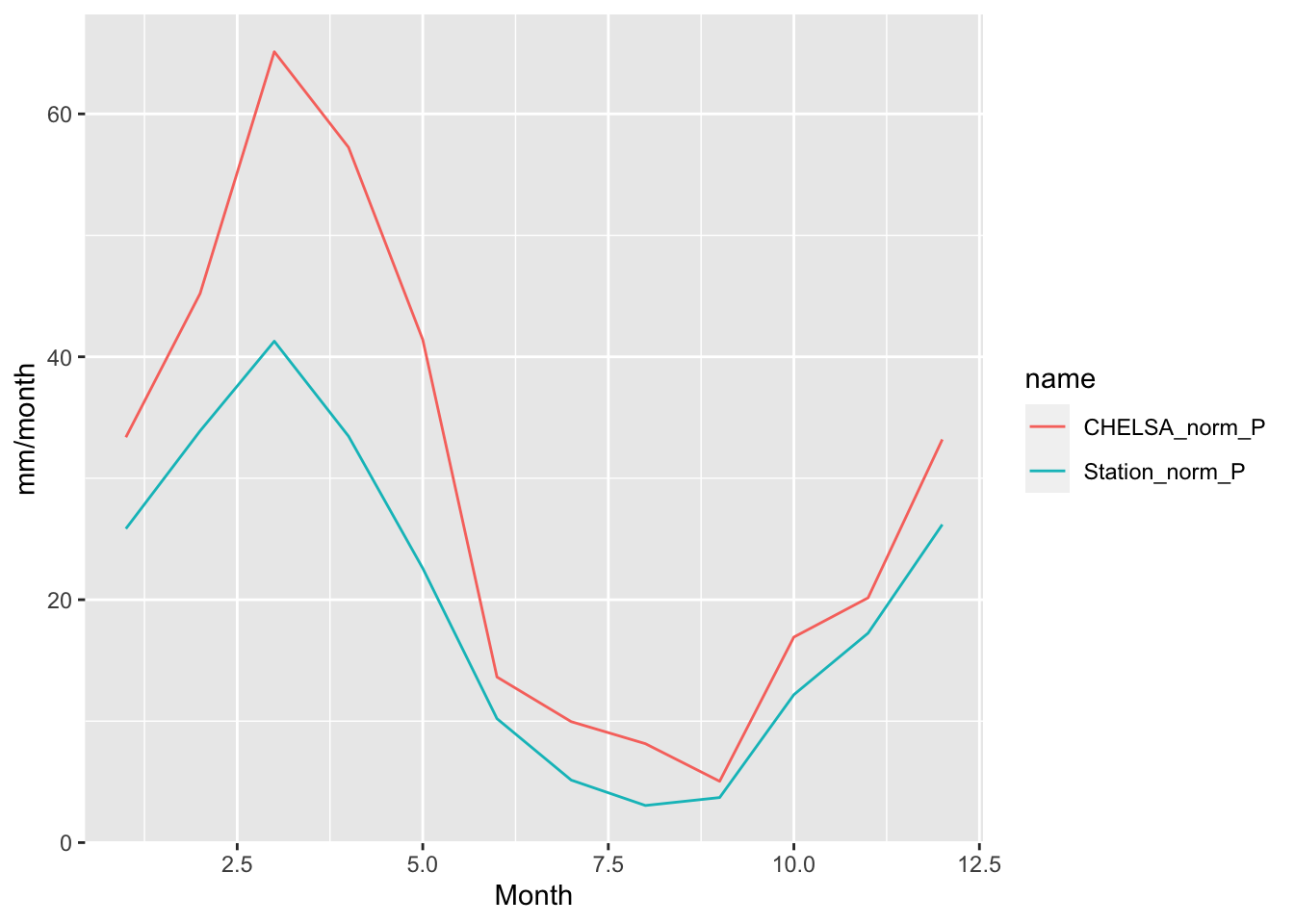

Figure 5.26: Monthly precipitation norms of the bias corrected CHELSA v1.2.1 dataset and the mean monthly precipitation averaged over the four meteorological stations in the Gunt river basin.

The seasonality of the precipitation is in excellent agreement between the observed data and the bias corrected CHELSA precipitation product. One should not be misled by the offset in absolute terms between the two datasets since since one is data derived from stations at particular locations and the other is average high-resolution gridded data.

A better way to plot the comparison of the seasonality of the two products would be to center and standardize the two datasets. This can be achieved the following way.

norm_P_data_zscore <- 
  norm_P_data %>% mutate(Station_norm_P_zscore = (Station_norm_P - mean(Station_norm_P))/ sd(Station_norm_P)) %>% 
  mutate(CHELSA_norm_P_zscore = (CHELSA_norm_P - mean(CHELSA_norm_P)) / sd(CHELSA_norm_P))
norm_P_data_zscore_long <- norm_P_data_zscore %>% dplyr::select(-Station_norm_P,-CHELSA_norm_P) %>% pivot_longer(-mon)
ggplot(norm_P_data_zscore_long,aes(x=mon,y=value,color = name)) + geom_line() + 
  xlab("Month") + ylab("[-]")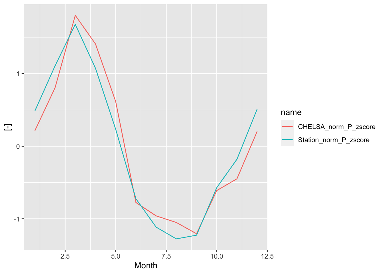

Figure 5.27: Centered and standardized precipitation norms for the comparison of the seasonality of the two products.The bias corrected CHELSA product reproduces the precipitation seasonlity in an excellent manner. Note that the values on the y-axis do not have any units as a result of the standarization.

To summarize, with the CHELSA v1.2.1 dataset, we have downloaded and prepared a high spatial resolution climatology for the Central Asia domain. As this product is derived from reanalysis data that mixes station data with climate model output, the precipitation product was bias corrected for snow undercatch that causes the original reanalysis data to greatly underestimate high-elevation precipitation data. As show for Gunt river basin in the Pamirs, the resulting temperature and precipitation climatologies compare in an excellent manner with seasonalities observed at local meteorological stations.

For hydrological modeling, however, we need not only high spatial resolution data but also high temporal resolution data, ideally at hourly time-steps, to drive the hydrological model. In the next Section @ref(Data::ERA5), we show how hourly ERA5 reanalysis data fields can be resampled and rescaled so that mean or total monthly values match CHELSA v.1.2.1 at particular raster cells. Like this, we will arrive at a dataset with high temporal and spatial resolution.

5.3.2 ERA5 Download and Data Resampling with PBCORR CHELSA

5.3.2.1 ERA5 Background

ERA5 data from 1981-01-01 through 2013-12-31 for the Central Asia domain is available for download under this link. Hourly temperature 2 meters above the surface (t2m) and hourly precipitation (tp) totals can be downloaded there⁹. More information about ERA5 data can be found on the official website of the European Center of Medium Weather Forecast.

With the Lobelia Past Climate Explorer, one can easily get key statistics of any of the ERA5 raster cells globally. Try it! Go to the Central Asia domain, search for your place of interest (i.e. your home, the Gunt river basin, Chirchik river basin, etc.) and click on the point where you would like to see the statistics. See also Figure 5.28

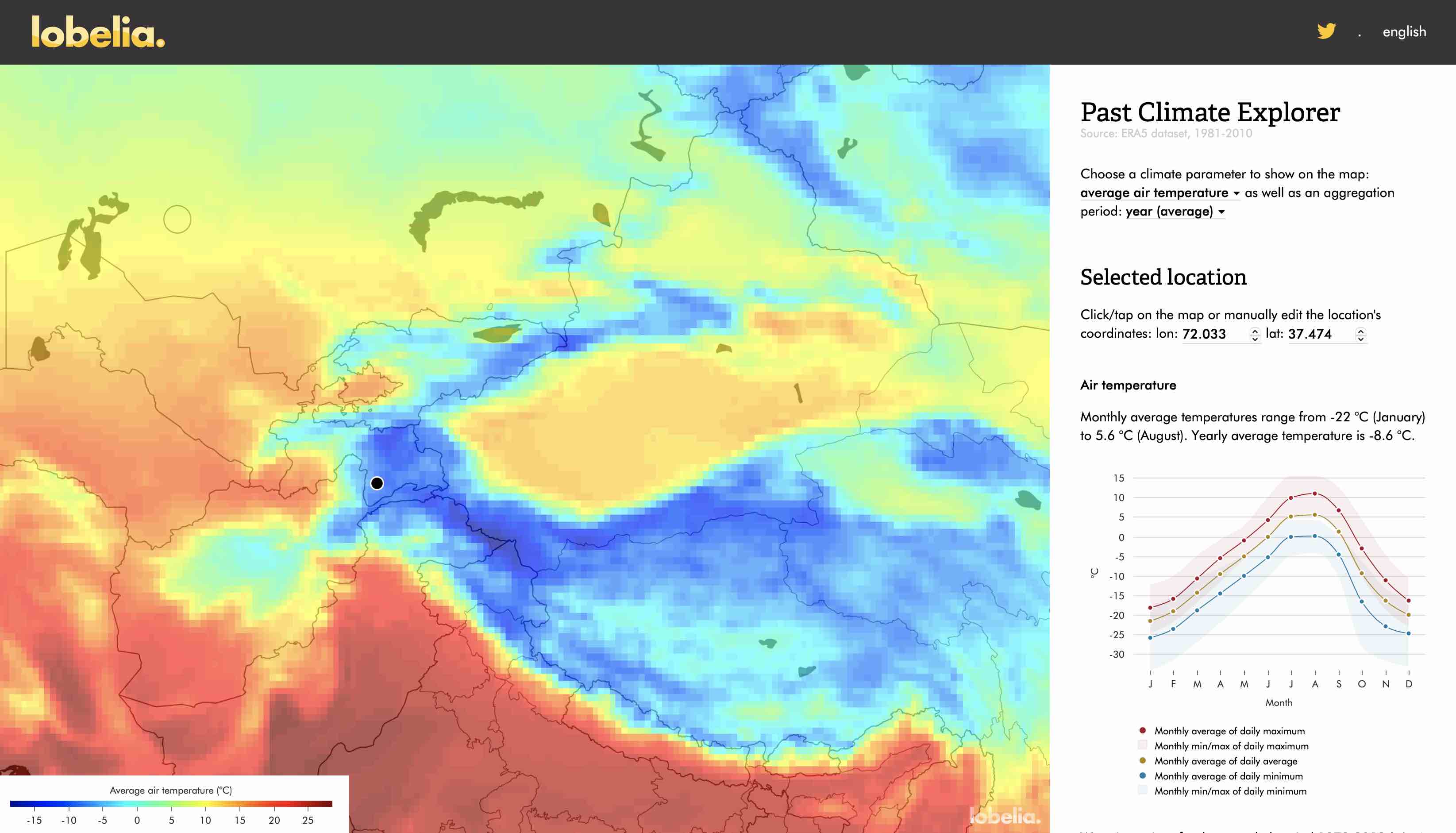
Figure 5.28: Screenshot from the Lovelia ERA5 website with the ERA5 temperature statistics of Khorog selected.

ERA5 data can be downloaded from the Copernicus Climate Change Service (C3S) Climate Data Store. We use the ERA5-Land hourly data from 1981 product. Note that if you want to download the data yourself from the Data Store, you need to register there.

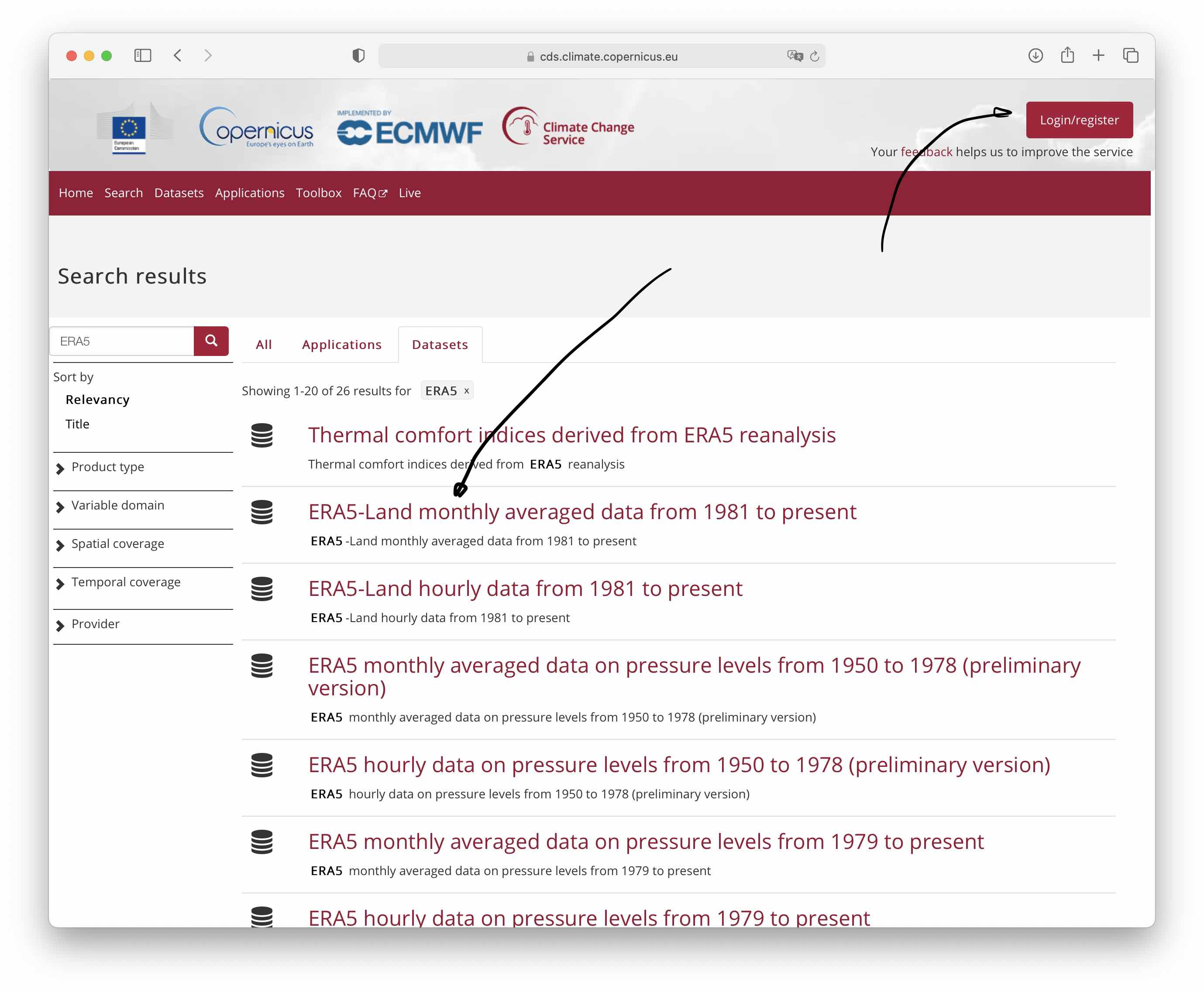
Figure 5.29: Screenshot from the Copernicus Climate Data Store. One needs to register first if you want to download data yourself from the Climate Data Store (click on Login/register button. The product which we download is highlighted. If you click on it, then the detailed data page comes up.

As per the ECMWF description, “ERA5-Land is a reanalysis dataset providing a consistent view of the evolution of land variables over several decades at an enhanced resolution compared to ERA5. ERA5-Land has been produced by replaying the land component of the ECMWF ERA5 climate reanalysis. Reanalysis combines model data with observations from across the world into a globally complete and consistent dataset using the laws of physics. Reanalysis produces data that goes several decades back in time, providing an accurate description of the climate of the past.” For more information, please visit the detailed data description webpage.

The variables t2m and tp which you can access via this link are described described in greater detail on the site. For reference, these data specifications are copied in the Table below.

ERA5-Land t2m and pr variables descriptions.

Name	Units	Description
2m temperature (t2m)	K	Temperature of air at 2m above the surface of land, sea or in-land waters. 2m temperature is calculated by interpolating between the lowest model level and the Earth’s surface, taking account of the atmospheric conditions. Temperature measured in kelvin can be converted to degrees Celsius (°C) by subtracting 273.15.
Total precipitation (tp)	m	Accumulated liquid and frozen water, including rain and snow, that falls to the Earth’s surface. It is the sum of large-scale precipitation (that precipitation which is generated by large-scale weather patterns, such as troughs and cold fronts) and convective precipitation (generated by convection which occurs when air at lower levels in the atmosphere is warmer and less dense than the air above, so it rises). Precipitation variables do not include fog, dew or the precipitation that evaporates in the atmosphere before it lands at the surface of the Earth. This variable is accumulated from the beginning of the forecast time to the end of the forecast step. The units of precipitation are depth in meters. It is the depth the water would have if it were spread evenly over the grid box. Care should be taken when comparing model variables with observations, because observations are often local to a particular point in space and time, rather than representing averages over a model grid box and model time step.

5.3.2.2 ERA5-Land Download

Note: This Section just demonstrates how you can order data from Copernicus Climate Data Store. It is not required for you to carry this out in order to access the Central Asia 2m temperature and total precipitation data that has been prepared for this course and is available for download here.

The manual data download from the Climate Data Store is tedious. We show here how, with an R-script, you can place a data order and then, once the data is prepared, download it from the Data Store.

The following code segments show to download daily ERA5 t2m and tp data that is segmented into yearly netCDF-files. Like this, these become manageable for later processing. Note that the two code segments start the scripts on the side of the Climate Data Store data service. Following the submission of jobs and after a wait of a couple of hours, the data can then be downloaded at https://cds.climate.copernicus.eu/cdsapp#!/yourrequests manually and stored in the relevant location. Note that for these scripts to run, you need to give your own credentials that you obtain after login in the Climate Data Store.

Under the assumption that you have typed in your credentials (user name, ID and key), 2 meter temperature data can be downloaded in the following way.

# Required library
library(ecmwfr)
# Prepare data download of ERA5 by adding login credentials to the keychain.
wf_set_key(user = '<Your user name>',
           key = "Your key",
           service = "webapi")


downloadList_t2m <- 1981:2013 # The years for which CHELSA v1.2.1 is available are chosen for download. These will be used for the calibration and vaildation of the hydrological model and constitute the reference hydrological period. 

for (yr in downloadList_t2m){
  CentralAsia_ERA5_hourly_request <- list(
    format = "netcdf",
    variable = c("2m_temperature"),
    year = as.character(yr),
    month = c("01", "02", "03", "04", "05", "06", "07", "08", "09", "10", "11", "12"),
    day = c("01", "02", "03", "04", "05", "06", "07", "08", "09", "10", "11", "12", "13", "14", "15", "16", "17", "18", "19", "20", "21", "22", "23", "24", "25", "26", "27", "28", "29", "30", "31"),
    time = c("00:00", "01:00", "02:00", "03:00", "04:00", "05:00", "06:00", "07:00", "08:00", "09:00", "10:00", "11:00", "12:00", "13:00", "14:00", "15:00", "16:00", "17:00", "18:00", "19:00", "20:00", "21:00", "22:00", "23:00"),
    area = c(45, 64, 34, 81),
    dataset_short_name = "reanalysis-era5-land",
    target = paste0("CentralAsia_ERA5_hourly_",as.character(yr),'.nc'))
  
  file <- wf_request(user     = "Your User ID",   # user ID (for authentication)
                     request  = CentralAsia_ERA5_hourly_request,  # the request name (can be anything)
                     transfer = FALSE,     # put it in the queue and download manually from the website
                     path     = ".",
                     job_name = paste0("t2m_CentralAsia_ERA5_hourly_",as.character(yr),'.nc'))  
}

Similarly, total precipitation is downloaded with the following code.

downloadList_tp <- 1981:2013

for (yr in downloadList_tp){
  CentralAsia_ERA5_hourly_request <- list(
    format = "netcdf",
    variable = c("total_precipitation"),
    year = as.character(yr),
    month = c("01", "02", "03", "04", "05", "06", "07", "08", "09", "10", "11", "12"),
    day = c("01", "02", "03", "04", "05", "06", "07", "08", "09", "10", "11", "12", "13", "14", "15", "16", "17", "18", "19", "20", "21", "22", "23", "24", "25", "26", "27", "28", "29", "30", "31"),
    time = c("00:00", "01:00", "02:00", "03:00", "04:00", "05:00", "06:00", "07:00", "08:00", "09:00", "10:00", "11:00", "12:00", "13:00", "14:00", "15:00", "16:00", "17:00", "18:00", "19:00", "20:00", "21:00", "22:00", "23:00"),
    area = c(45, 64, 34, 81),
    dataset_short_name = "reanalysis-era5-land",
    target = paste0("CentralAsia_ERA5_hourly_",as.character(yr),'.nc'))
  
  file <- wf_request(user     = "11732",   # user ID (for authentication)
                     request  = CentralAsia_ERA5_hourly_request,  # the request
                     transfer = FALSE,     # put it in the queue and download manually from the website
                     path     = ".",
                     job_name = paste0("tp_CentralAsia_ERA5_hourly_",as.character(yr),'.nc'))  
}

5.3.2.3 Rescaling ERA5 to monthly CHELSA values

ERA5 original data can easily be rescaled (bias corrected) to CHELSA data values for any river basin in the Central Asia domain using the convenience function riversCentralAsia::biasCorrect_ERA5_CHELSA(). Type ?biasCorrect_ERA5_CHELSA to get more information about the function and its arguments. The code block below shows how to rescale (bias correct) total precipitation. It assumes that the ERA5 directory contains two subfolders ERA5/tp/ and ERA5/t2m where the corresponding data are stored.

# Specify biasCorrect_ERA5_CHELSA() function arguments
basinName <- 'Gunt'
dataType_ERA5 <- 'tp' # note that ERA5 tp units are in m!
## Directories of relevant climate files  - function arguments
dir_ERA5_hourly <- '../HydrologicalModeling_CentralAsia_Data/CentralAsiaDomain/ERA5/'
dir_CHELSA <- '../HydrologicalModeling_CentralAsia_Data/CentralAsiaDomain/CHELSA_V1.2.1/'
# start and end times - function arguments
startY <- 1981
endY <- 2013

biasCorrect_ERA5_CHELSA(dir_ERA5_hourly,dataType_ERA5,dir_CHELSA,startY,endY,basinName,gunt_Shapefile_LatLon)

By simply switching the data type (effectively, it just looks for the files in the corresponding directory), temperature can be rescaled to the CHELSA field values for each month.

# Specify biasCorrect_ERA5_CHELSA() function arguments
basinName <- 'Gunt'
dataType_ERA5 <- 't2m' # note that ERA5 tp units are in m!
## Directories of relevant climate files  - function arguments
dir_ERA5_hourly <- '../HydrologicalModeling_CentralAsia_Data/CentralAsiaDomain/ERA5/'
dir_CHELSA <- '../HydrologicalModeling_CentralAsia_Data/CentralAsiaDomain/CHELSA_V1.2.1/'
# start and end times - function arguments
startY <- 1981
endY <- 2013

biasCorrect_ERA5_CHELSA(dir_ERA5_hourly,dataType_ERA5,dir_CHELSA,startY,endY,basinName,gunt_Shapefile_LatLon)

In order to understand if the rescaling of the ERA5 data lead to meaningful results, we can compare monthly precipitation totals from the final ERA5 data to monthly station values, average over the four meteorological stations that we have.

basinName <- 'Gunt'
dataType_ERA5 <- 'tp' # note that ERA5 tp units are in m!
## Directories of relevant climate files  - function arguments
dir_ERA5 <- '../HydrologicalModeling_CentralAsia_Data/CentralAsiaDomain/ERA5/' # Note: ERA5 data in m
# basin
basin_shp_latlon <- gunt_Shapefile_LatLon
# start and end times - function arguments
startY <- 1981
endY <- 2013
# Date sequence
sTime <- paste0(startY,'-01-01 01:00:00')
eTime <- paste0(endY,'-12-31 23:00:00')
dateSeq_ERA <- seq(as.POSIXct(sTime), as.POSIXct(eTime), by="hour")
dateSeq_ERA <- tibble(date=dateSeq_ERA, data=NA)
dateSeq_ERA <- dateSeq_ERA %>% mutate(month = month(date)) %>% mutate(year = year(date))
# Create Basin subdirectory (if not already existing) to store dedicated annual files there
mainDir <- paste0(dir_ERA5,dataType_ERA5,'/',basinName,'/')
# Start data fetching
for (yr in startY:endY){
  # progress indicator
  print(paste0('PROCESSING YEAR ',yr))
  # file handling
  file2Process_ERA <- paste0(dataType_ERA5,'_ERA5_hourly_',basinName,'_bcorr_',yr,'.nc')
  era_data<- brick(paste0(mainDir,file2Process_ERA))
  # extract the data over the basin
  dateSeq_ERA$data[dateSeq_ERA$year==yr] <- raster::extract(era_data,basin_shp_latlon,fun=mean)
}

dateSeq_ERA_mon <- dateSeq_ERA %>% dplyr::select(date,data) 

if (dataType_ERA5=='t2m'){
  era5_data_mon <- dateSeq_ERA_mon %>% timetk::summarize_by_time(.date_var = date,.by = 'month',era5_data_mon = mean(data),.type = 'ceiling')
  station_data_mon <- data %>% filter(type=='mean(T)' & resolution=='mon') %>%
    dplyr::select(date,data,code) %>%
    filter(date>=(dateSeq_ERA_mon$date %>% first())) %>% 
    filter(date<=(dateSeq_ERA_mon$date %>% last())) %>% 
    pivot_wider(names_from = 'code',values_from = data) %>% 
    mutate(station_data_mon = rowMeans(dplyr::select(.,-date),na.rm=TRUE)) %>% 
    dplyr::select(date,station_data_mon)
} else {
  era5_data_mon <- dateSeq_ERA_mon %>% timetk::summarize_by_time(.date_var = date,.by = 'month',era5_data_mon = sum(data),.type = 'ceiling')
  era5_data_mon$era5_data_mon <- era5_data_mon$era5_data_mon * 1000 # in mm now
  station_data_mon <- data %>% filter(type=='P' & resolution=='mon') %>%
    dplyr::select(date,data,code) %>%
    filter(date>=(dateSeq_ERA_mon$date %>% first())) %>% 
    filter(date<=(dateSeq_ERA_mon$date %>% last())) %>% 
    pivot_wider(names_from = 'code',values_from = data) %>% 
    mutate(station_data_mon = rowMeans(dplyr::select(.,-date),na.rm=TRUE)) %>% 
    dplyr::select(date,station_data_mon)
  
}
era5_data_mon$date <- (era5_data_mon$date - 3600) %>% as.Date()
data_validation <- full_join(era5_data_mon,station_data_mon,by='date')
data_validation %>% pivot_longer(-date) %>% 
  plot_time_series(.date_var = date,.value = value,.smooth = FALSE,
                   .color_var = name,.title = "",.x_lab = "Year",.y_lab = "mm/month",.interactive = FALSE)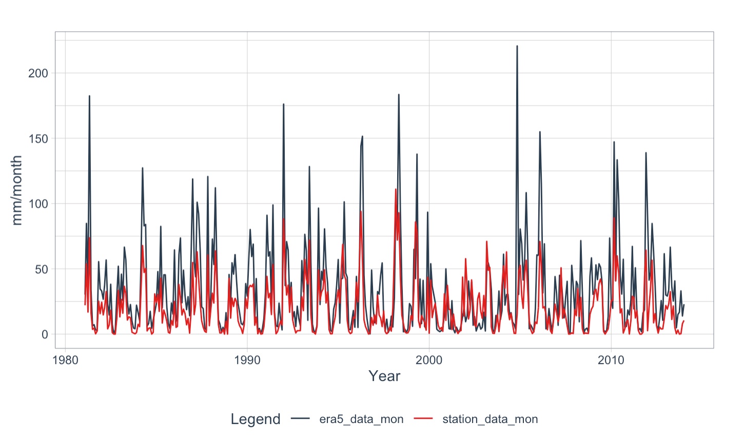

Figure 5.30: Comparison of mean monthly precipitation values of the Gunt meteorlogical Stations with the rescaled ERA5 data in the basin. The timeseries compare favorably, both in terms of seasonality and interannual variability.

5.3.2.4 Downscaling ERA5 to Basin Elevation Bands and Data Export to RS MINERVE Database file

The next and last step for the preparation of the input data required for hydrological modeling in RS MINVERVE involves the downscaling of the prepared hourly ERA5 data to the individual subbasins and elevation bands inside a catchment. The process of generating the input files is shown by using data from the Gunt river basin.

The Gunt river basin outline is shown in Figure 5.31. We want to downscale the prepared hourly ERA5 climate fields over the domain of the Gunt river basin to the individual subbasins and the elevation bands of these subbasins (see Figures 5.31 to ?? below). In other words, we want to generate hourly climate timeseries of mean temperature and precipitation levels for each subbasin and all of the elevation bands in each subbasin. The hydrological processes of each of these subbasin elevation bands will then be modeled with a separate model. All these individual hydrological models will be interconnected according to the existing flow topology in the basin. Like this, we arrive at a lumped (lumped over the subbasin-specific elevation bands), semi-distributed (distributed between the subbasins and elevation bands) hydrological model of the entire catchment.

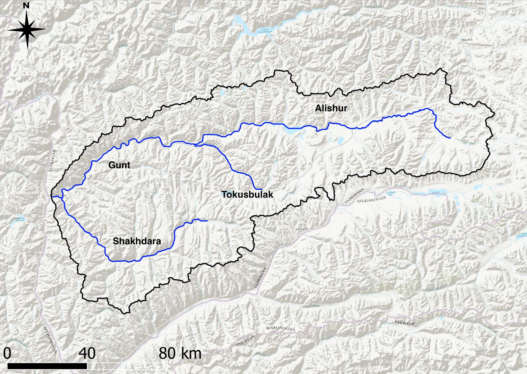
Figure 5.31: The outline of the Gunt river catchment is shown with the key river sections of all tributariies from the corresponding subbasins.

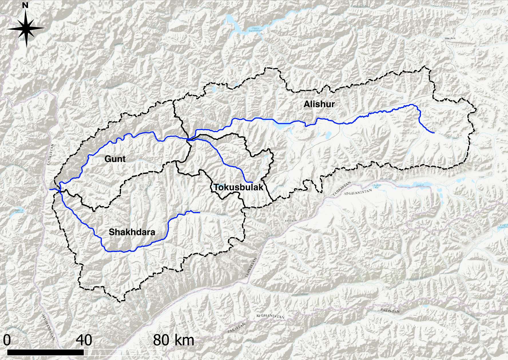
Figure 5.32: Gunt river catchment with the individual subbasins is shown. These subbasins are further divided into elevation band zones and the mean climate finally extracted over these subbasin-specfic elevation bands (see Figure (ref?)(fig:guntSubasinsElevationBands)).

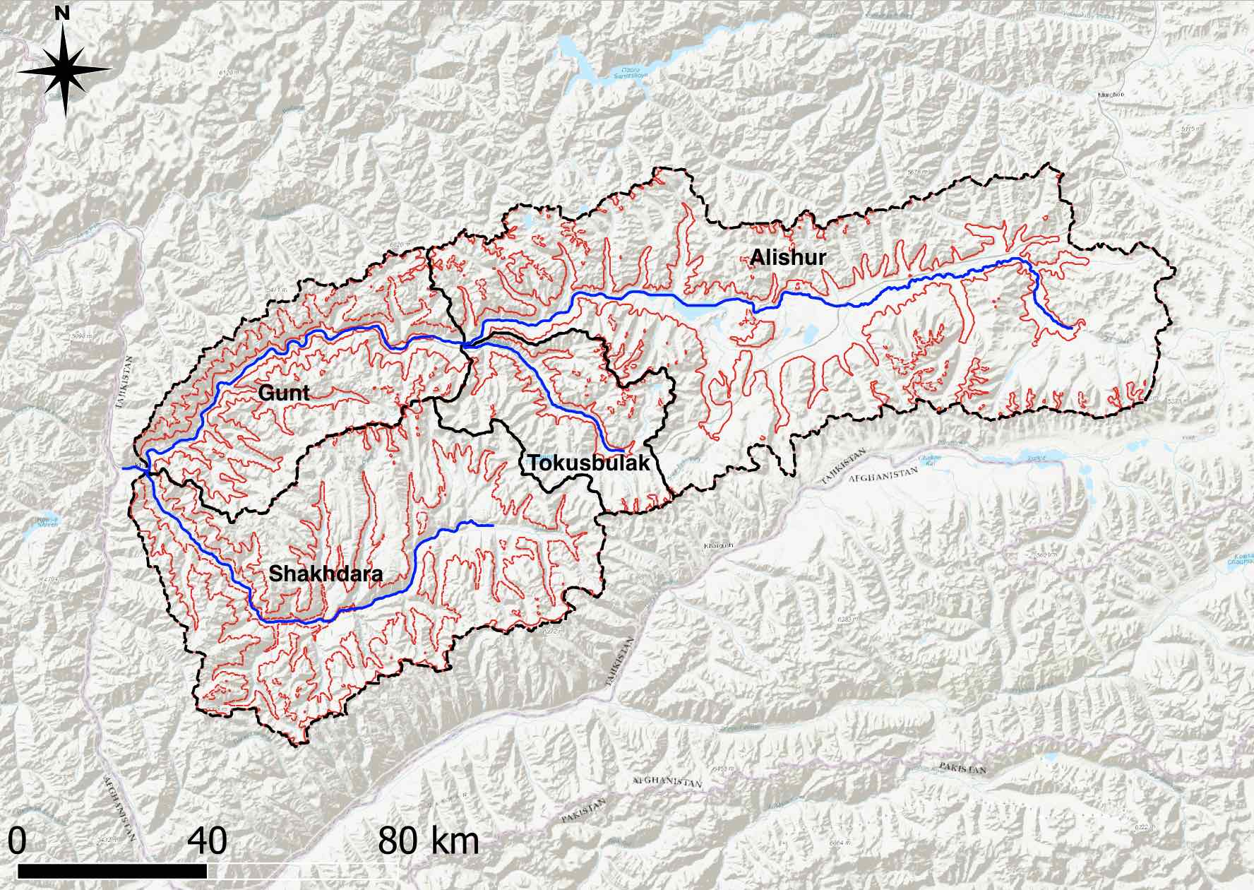
Figure 5.33: The Gunt river catchment elevation bands are shown in red color. The entire catchment was divided into 4 altitude zones with an interval spacing of 1’000 meters. In real world climate impact studies, elevation bands are normally generated with an interval spacing of 200 - 500 meters.

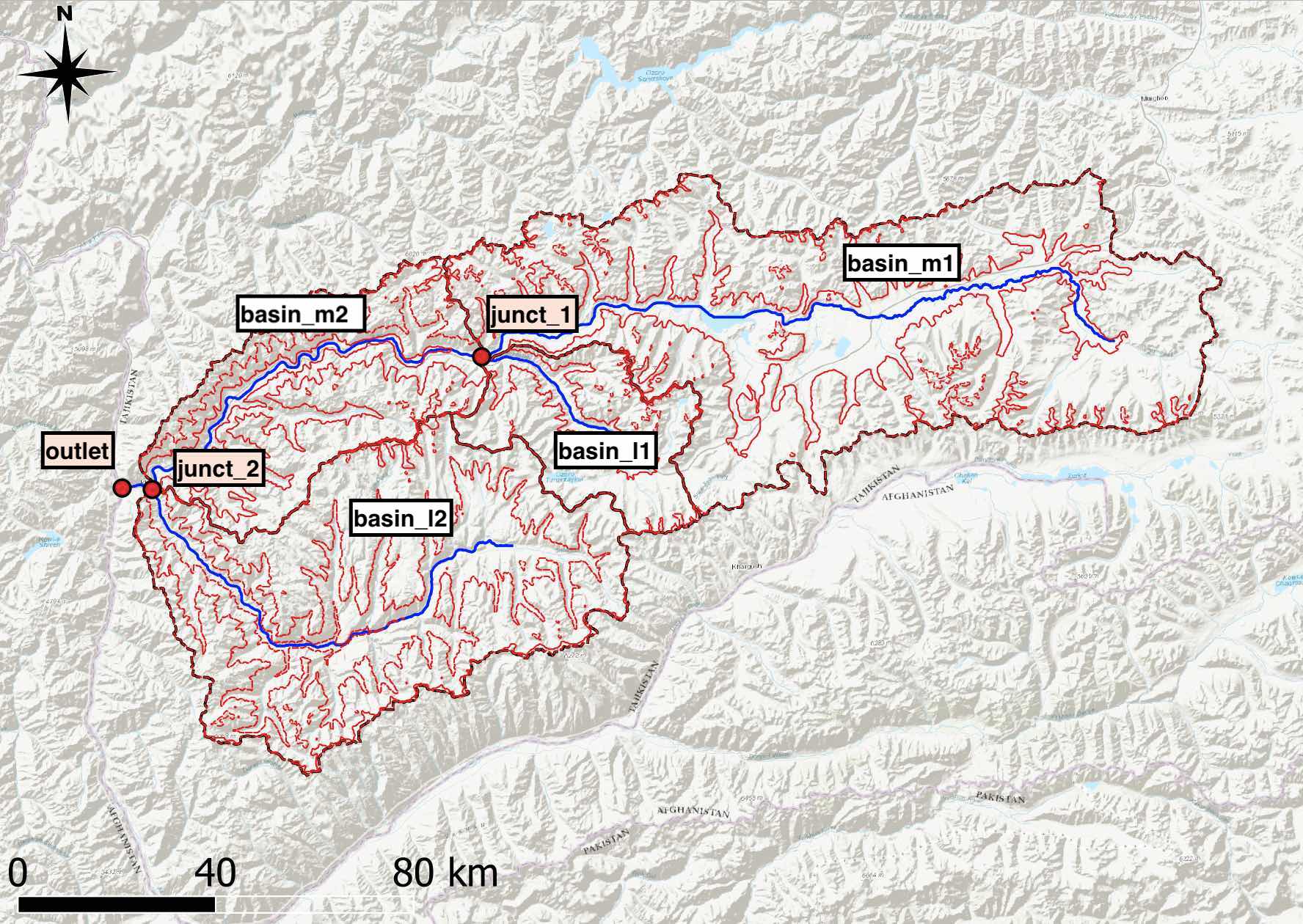
Figure 5.34: The naming concention of the subbasins is shown. For each subbasin, the bands are identified with a suffix .._b1 for elevation band 1, .._b2 for elevation band 2 and so on.

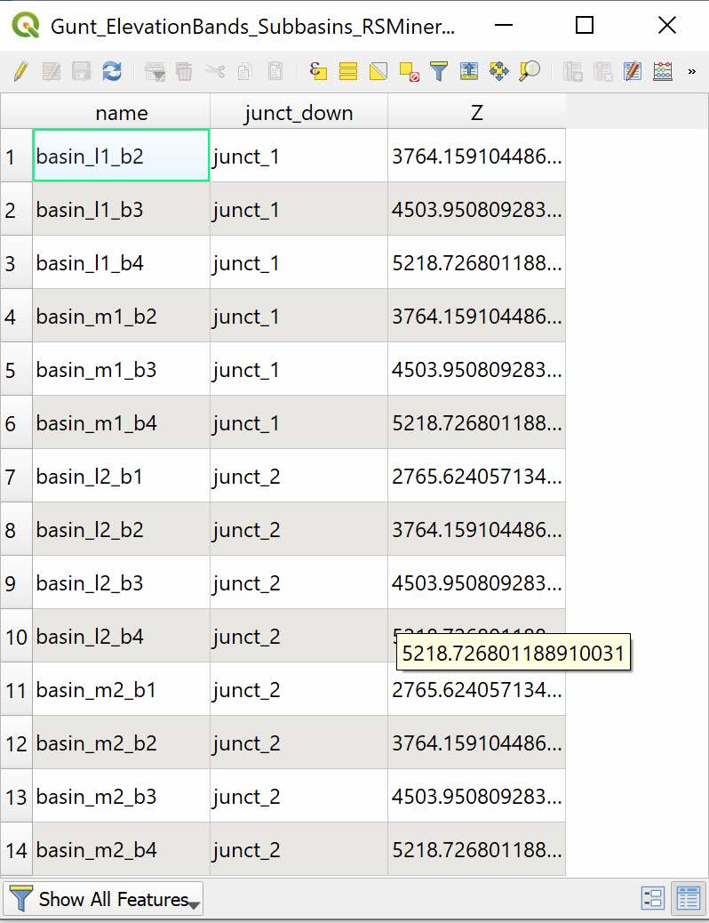
Figure 5.35: Subbasin elevation band attribute table. In total there are 14 elevation bands and for each elevation band, a climate time series is created with the function riversCentralAsia::generate_ERA5_Subbasins_CSV(). The Z field is important and specifies the average elevation of the corresponding elevation band for each subbasin.

The code block assumes that the previously described steps have been carried and that the corresponding files are stored in the correct relative path locations. First, ERA5 precipitation is downscaled with generate_ERA5_Subbasin_CSV(...) with dataType='tp' set. Second, dataType='t2m' for the downscaling of the 2 meter above surface ERA5 temperature. In a third step, we add the discharge data to the resulting data frame in the last column. Finally, the observed discharge data is added. Note here that we add the gap filled time series of the observational record. The process of gap filling discharge data is described in Section 5.1.2 above.

# Housekeeping
dir_ERA5 <- '../HydrologicalModeling_CentralAsia_Data/CentralAsiaDomain/ERA5/'
catchmentName <- 'Gunt'
elBands_shp <- st_read('../HydrologicalModeling_CentralAsia_Data/AmuDarya/Gunt/GeospatialData/Gunt_ElevationBands_Subbasins_RSMinerve.shp')

startY <- 1981
endY <- 2013

# 1. Downscaling precipitation
dataType <- 'tp' # Precipitation
gunt_db_tp <- generate_ERA5_Subbasin_CSV(dir_ERA5_hourly,catchmentName,dataType,elBands_shp,startY,endY)
# 2. Downscaling temperature
dataType <- 't2m' # Temperature
gunt_db_t2m <- generate_ERA5_Subbasin_CSV(dir_ERA5_hourly,catchmentName,dataType,elBands_shp,startY,endY)
# 3. Joining the two data frames.
gunt_db <- gunt_db_t2m %>% add_column(gunt_db_tp %>% dplyr::select(-Station),.name_repair = 'unique') 
# 4. Adding the observed discharge data in the required format to the data frame
gunt_db_Q <- q_17050_mon_filled %>% dplyr::select(date,data) 
gunt_db_Q$date <- gunt_db_Q$date %>% as.POSIXct() + 22 * 60 * 60 # just adding time so that we are indeed at the end of the month 
datesChar_Q <- posixct2rsminerveChar(gunt_db_Q$date) %>% rename(Station=value)
datesChar_Q <- datesChar_Q %>% add_column(Q_17050 = (gunt_db_Q$data %>% as.character))

gunt_db_Q <- full_join(gunt_db,datesChar_Q,by='Station') # this works well
# now finish off by giving the required attributes in the table for the discharge station
gunt_db_Q$Q_17050[1] = 'Q_17050'
gunt_db_Q$Q_17050[2] = meteoStations$utm.x[2]
gunt_db_Q$Q_17050[3] = meteoStations$utm.y[2]
gunt_db_Q$Q_17050[4] = meteoStations$masl[2]
gunt_db_Q$Q_17050[5] = 'Q'
gunt_db_Q$Q_17050[6] = 'Flow'
gunt_db_Q$Q_17050[7] = 'm3/s'
gunt_db_Q$Q_17050[8] = 'Constant before'

The resulting data frame can be stored with write.table(..,..,sep=',',row.names = FALSE,col.names=FALSE,quote=FALSE) as a csv-file and the read into RS MINERVE later. A screenshot of the csv-file is below in Figure 5.36. Elevation band-specific temperature (T) and precipitation (P) data are stored in columns. The last column contains the discharge data Q. If more than one observation station are available, more discharge columns would correspondingly need to be added.

In row 1 - 8, elevation band specific information is stored. More specifically, the following information is contained:

• Row 1: Name of elevation band and discharge station(s)

• Row 2: Longitude of centroid of elevation band and location of gauging station(s) (in meters, UTM)

• Row 3: Latitude of centroid of elevation band and location of gauging station(s) (in meters, UTM)

• Row 4: Mean elevation across elevation band and elevation of gauging station(s)

• Row 5: Observation type indicator (T: temperature, P: precipitation and Q: discharge)

• Row 6: Category

• Row 7: Measurement units

• Row 8: Interpolation method for downsampling course resolution time series¹⁰

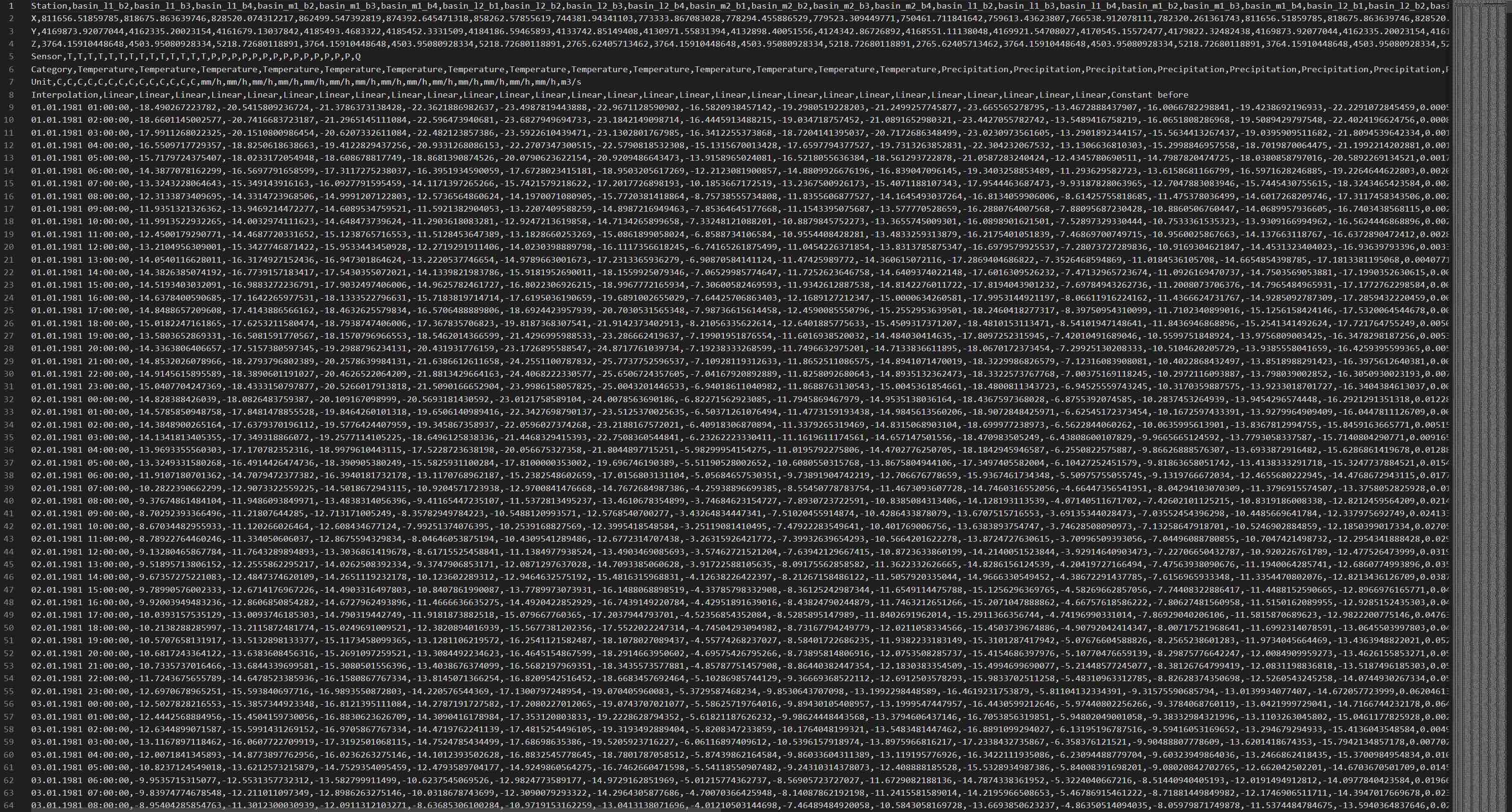
Figure 5.36: Screenshot of the resulting large csv file that can be read into RS MINERVE.

From rows 9 onward, the actual data are stored where a time stamp in the first column corresponds to the corresponding observation data and time.

---

7. Please note that the total size of this repository is 2 GB, approximately. Prior to downloading these data, you should ensure that you have enough storage space on your local machine. Furthermore, it is advised that you create the directory structure in the following way:

   FILES/PROJECT
   -Code
   —yourRProject.Rproj
   —code1.R
   —…
   -HydrologicalModeling_CentralAsia_Data
   —
   

   where FILES/PROJECT is the folder where you keep your documents on your computer and project denotes the folder name of your project, Code is the folder where all your code lives and HydrologicalModeling_CentralAsia_Data is the folder where you store all the accompanying data that can downloaded.↩︎

8. The code for the computation of the CHELSA long-term monthly mean temperature and precipitation climatologies is provided in the Appendix C in the corresponding Sect.↩︎

9. Please note that one raster brick that encompasses the data for one year is approx 333 MB to download!↩︎

10. This is for example used to downsample monthly discharge as provided by the hydrometeorological agency to hourly discharge (we use hourly simulation time steps in the hydrological model).↩︎