6.4 Data Preparation and Setup
The data used in this Chapter can be accessed on the public GitHub repository Applied Modeling of Hydrological Systems in Central Asia and the ./data/AmuDarya/Gunt/ folder in there. It is advisable that the user downloads the data and sets up a similar data directory structure on their local machines.
6.4.1 Examining and Understanding the GIS Data
As demonstrated in the Examples of the User Manual, RS Minerve does not necessarily require GIS input files for setting up models. These can also be setup and wired by hand. However, individual subbasins that contribute to flow in a larger catchment have different characteristics that need to be derived from spatial data, i.e. GIS files. For example, subbasin areas, river stretch lengths, terrain slopes, etc., are all required data in an RS Minerve model. These data could either be typed in by hand for each subbasin or automatically inserted via the GIS Import option. The latter method is much more convenient and is demonstrated here16.
First, we load the required packages in R.
# Loading required packages
## Tidy data wrangling
library(tidyverse)
library(here)
library(timetk)
library(tidymodels)
library(lubridate)
library(timetk)
## riversCentralAsia Package
library('riversCentralAsia')
## Spatial data processing
library(raster)
library(sf)
Now, we can visualize the GIS files that are required in RS Minerve in the following Figure 6.6.
# Load data
fPath <- './data/AmuDarya/Gunt'
gunt_DEM <- raster(paste0(fPath,'/GeospatialData/17050_Gund_Basin_DEM.tif'))
gunt_elBands_shp_utm <- st_read(paste0(fPath,'/GeospatialData/Gunt_ElevationBands_Subbasins_RSMinerve.shp'),quiet=TRUE)
gunt_subbasins_shp_utm <- st_read(paste0(fPath,'/GeospatialData/Gunt_Subbasins_RSMinerve.shp'),quiet=TRUE)
gunt_subbasin_junctions_shp_utm <- st_read(paste0(fPath,'/GeospatialData/Gunt_Junctions_RSMinerve.shp'),quiet=TRUE)
gunt_rivers_shp_utm <- st_read(paste0(fPath,'/GeospatialData/Gunt_Rivers_RSMinerve.shp'),quiet=TRUE)

# Downsample DEM and create hillshade
gunt_DEM_lr <- raster::aggregate(gunt_DEM,fact=10) # this is in UTM 42N
gunt_slope <- terrain(gunt_DEM_lr, opt='slope')
gunt_aspect <- terrain(gunt_DEM_lr, opt='aspect')
gunt_DEM_hillshade <- hillShade(gunt_slope, gunt_aspect, 40, 270)

# Convert to dataframe for ggplotting
gunt_DEM_spdf <- as(gunt_DEM_lr, "SpatialPixelsDataFrame")
gunt_DEM_df <- as.data.frame(gunt_DEM_spdf)
colnames(gunt_DEM_df) <- c("value", "x", "y")
hillshade_Gunt_spdf <- as(gunt_DEM_hillshade, "SpatialPixelsDataFrame")
hillshade_Gunt_df <- as.data.frame(hillshade_Gunt_spdf)
colnames(hillshade_Gunt_df) <- c("value", "x", "y")

# Used for subbasins naming
subbasins <- # just put everything in a regular dataframe
  tibble(basin=c("Shakhdara","Gunt","Tokusbulak","Alishur"),
         lat   = c(37.4,37.75,37.6,37.65),
         lon   = c(72.0,71.8,72.6,73.25))
subbasins_coord_latlon = SpatialPoints(cbind(subbasins$lon, subbasins$lat), proj4string=CRS("+proj=longlat"))
subbasins_coord_UTM <- spTransform(subbasins_coord_latlon, CRS("+init=epsg:32642")) %>%
  coordinates() %>% as_tibble() %>%
  rename(x=coords.x1,y=coords.x2)
subbasins <- bind_cols(subbasins,subbasins_coord_UTM)
# Plotting
ggplot() +
  geom_tile(data=gunt_DEM_df, aes(x=x, y=y, fill=value), alpha=0.8) +
  geom_sf(data=gunt_subbasins_shp_utm,color="black",fill=NA,linetype="11",size=0.25) +
  geom_sf(data=gunt_rivers_shp_utm,color="blue",fill=NA) +
  geom_sf(data=gunt_elBands_shp_utm,color="black",fill=NA,linetype="11",size=.2) +
  geom_sf(data=gunt_subbasin_junctions_shp_utm,color="red",fill="red") +
  scale_fill_gradientn(colours = terrain.colors(100)) +
  xlab("Longitude") + ylab("Latitude") +
  guides(fill=guide_legend(title="Alt. [masl]")) +
  ggtitle("Gunt catchment and subbasins") +
  geom_label(data = subbasins,aes(x = x, y = y, label = basin),vjust = 0,hjust = 0)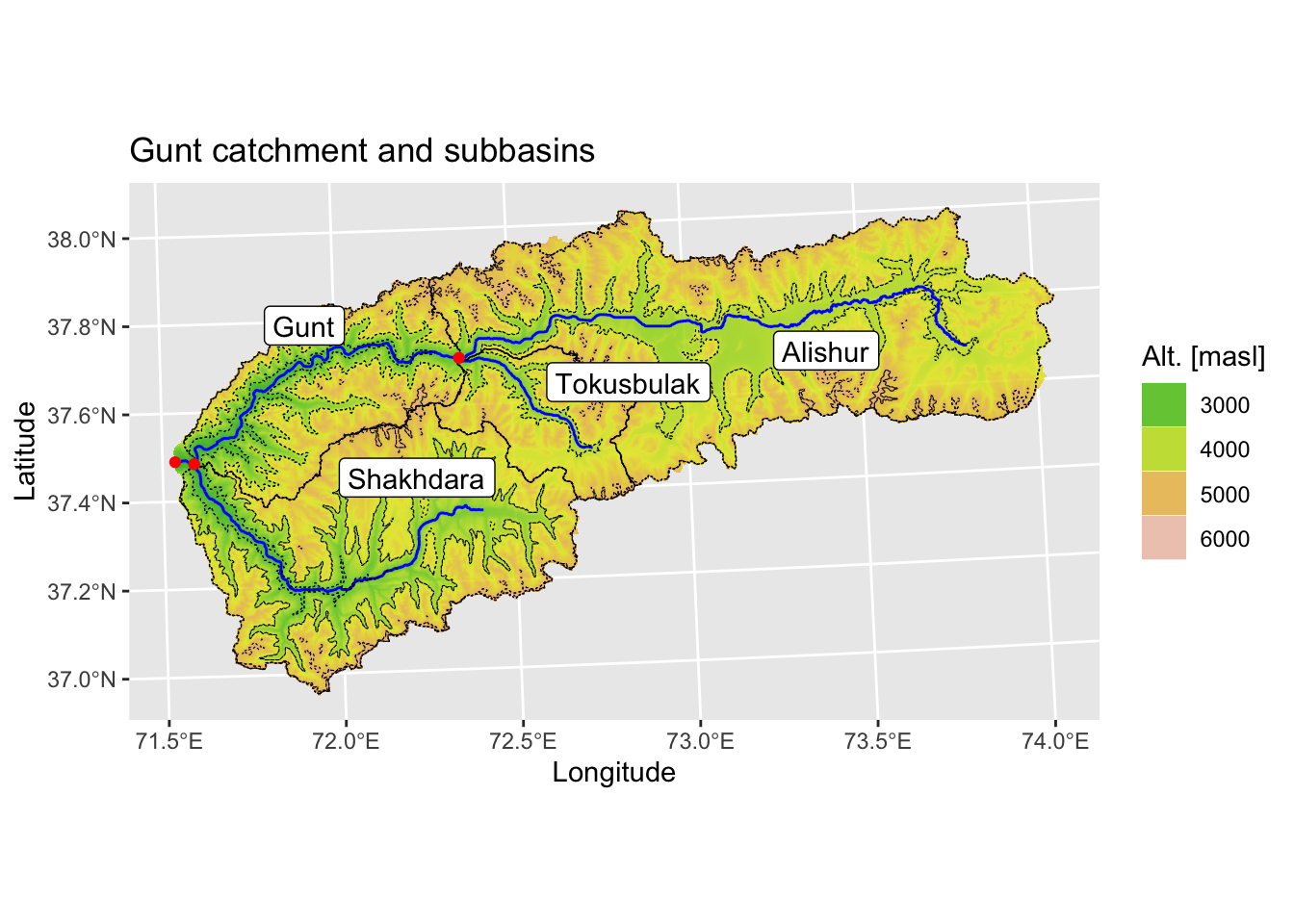
Figure 6.6: Gunt river basin overview, showing the digital elevation model, the 4 subcatchments, the elevation bands with 1’000 meters intervals, the main tributary rivers and the corresponding junctions.
Figure 6.6 shows the four subbasins. After the confluence with Tokusbulak river, Alishur river becomes Gunt river in Junction 1 (called junct_1 in the corresponding shapefile below). The confluence is noted by the corresponding red dot. Further downstream, approximately 5 km before the Gunt-Khorog gauging station (Hydromet Code 17050), indicated by the leftmost outlet point (red dot, called junct_2 in the junct_down attribute field of the shapefile), Shakhdara river feeds into Gunt. The subbasin-specific elevation bands are indicated by dotted lines.
As described in the RS Minerve User Manual in Chapter 5 (Foehn et al. 2020), the following three shapefiles need to be prepared for later loading into RS Minerve: subbasins.shp, junctions.shp and rivers.shp (see Figure 6.7).
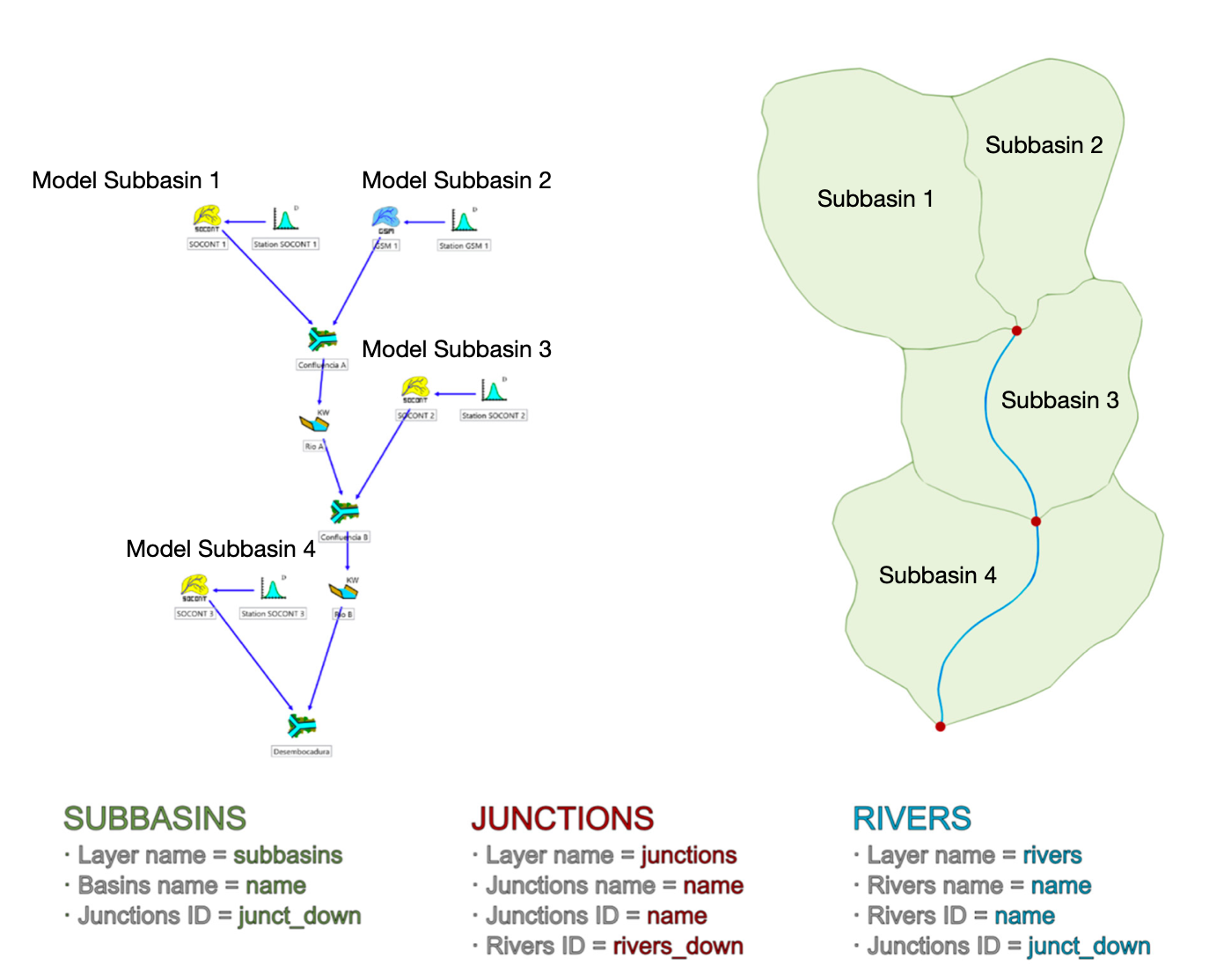
Figure 6.7: Required GIS input files for RS Minerve. See corresponding user manual for more information.
The shapefile attributes that you downloaded of the required data can easily be displayed. First, we analyze the subbasins `gunt_elBands_shp_utm` file. The file contains the following attributes as per the requirements specified in Figure 6.7: name and junct_down. The attributes Z, ModelGuid and geometry are additional fields. The field Z that contains information of the mean elevation of the subbasin. Note that the shapefile is does not only contain the shape of the four subbasins Alishu, Tokusbulak, Gunt and Shakdara but also the elevation bands of each subbasin.
# view meta data summary of the subbasins file
gunt_elBands_shp_utm <- sf::st_read(paste0(fPath,'/GeospatialData/Gunt_ElevationBands_Subbasins_RSMinerve.shp'),quiet=TRUE)
gunt_elBands_shp_utm
## Simple feature collection with 14 features and 3 fields
## Geometry type: MULTIPOLYGON
## Dimension: XY
## Bounding box: xmin: 725348.3 ymin: 4093789 xmax: 945535.6 ymax: 4216482
## Projected CRS: WGS 84 / UTM zone 42N
## First 10 features:
## name junct_down Z geometry
## 1 basin_l1_b2 junct_1 3764.159 MULTIPOLYGON (((796644.2 41...
## 2 basin_l1_b3 junct_1 4503.951 MULTIPOLYGON (((827142.4 41...
## 3 basin_l1_b4 junct_1 5218.727 MULTIPOLYGON (((827592.4 41...
## 4 basin_m1_b2 junct_1 3764.159 MULTIPOLYGON (((801343.9 41...
## 5 basin_m1_b3 junct_1 4503.951 MULTIPOLYGON (((838641.8 41...
## 6 basin_m1_b4 junct_1 5218.727 MULTIPOLYGON (((840091.7 41...
## 7 basin_l2_b1 junct_2 2765.624 MULTIPOLYGON (((727648.2 41...
## 8 basin_l2_b2 junct_2 3764.159 MULTIPOLYGON (((726448.3 41...
## 9 basin_l2_b3 junct_2 4503.951 MULTIPOLYGON (((757446.5 40...
## 10 basin_l2_b4 junct_2 5218.727 MULTIPOLYGON (((760396.3 40...This is because in RS Minerve, we will model each elevation zone of each subbasin with a separate rainfall-runoff model. These are then linked to each other via the topological ordering that is given by the rivers and junctions. The naming of the subbasins is somewhat arbitrary and tailored to the particular catchment under consideration. The prefix ‘basin_’ is everywhere the same. The basic idea is to identify a main river stem (denoted with mX) where the X is a number that increases from 1 towards the downstream after each confluence with a right or left tributary. In our case, Alishur river is denoted with m1. Gunt river, which emerges after the confluence with Tokusbulak (see Figure 6.6), is denoted with m2. Finally, Gunt river after the confluence with Shakhdara is m3. Each left tributary is denoted with lX and each right tributary with rX, where X is again a number starting from 1 and gradually increasing. In our case, Tokusbulak thus is l1 (the first left tributary joining the main river). Finally, Shakhdara is l2. Note, in the Gunt river basin, we do not have major right tributaries.
‘m1_b2’ the refers to the main upstream river, Alishur in this case, and its elevation band 2. m1_b3 would then be the third elevation band accordingly and so on. Why is there no m1_b1 feature? This is simple to understand. Since the entire basin is subdivided into n equally spaced elevation zones, the higher lying subbasins might no longer contain all elevation bands. For both, Alishur (main m1) and Tokusbulak (l1) this is the case where band b1 is simply not represented because of the high elevations of the subbasins.
#  view meta data summary of the junctions file
gunt_subbasin_junctions_shp_utm <- sf::st_read(paste0(fPath,'/GeospatialData/Gunt_Junctions_RSMinerve.shp'),quiet=TRUE)
gunt_subbasin_junctions_shp_utm
## Simple feature collection with 3 features and 2 fields
## Geometry type: POINT
## Dimension: XYZM
## Bounding box: xmin: 724198.4 ymin: 4151736 xmax: 795694.3 ymax: 4178534
## z_range: zmin: 2074.126 zmax: 3118.366
## m_range: mmin: 0 mmax: 0
## Projected CRS: WGS 84 / UTM zone 42N
## name river_down geometry
## 1 junct_2 gunt_ds POINT ZM (728998.1 4151736 ...
## 2 junct_3 <NA> POINT ZM (724198.4 4152236 ...
## 3 junct_1 gunt_us POINT ZM (795694.3 4178534 ...For the junctions shapefile, we define their names as well the field river_down, i.e. the name of the river downstream of the junction. Finally, for the rivers shapefile, we define the rivers name and the downstream junction junct_down. The terminal junction corresponds to the outlet of the model. It can be easily seen that junct_3 is the outlet since there is no more downstream river, i.e. <NA>.
# view meta data summary of the rivers file
gunt_rivers_shp_utm <- st_read(paste0(fPath,'/GeospatialData/Gunt_Rivers_RSMinerve.shp'),quiet=TRUE)
gunt_rivers_shp_utm
## Simple feature collection with 5 features and 3 fields
## Geometry type: LINESTRING
## Dimension: XYZM
## Bounding box: xmin: 724198.4 ymin: 4119538 xmax: 923686.9 ymax: 4196533
## z_range: zmin: 2074.126 zmax: 4040.01
## m_range: mmin: -1.797693e+308 mmax: 0
## Projected CRS: WGS 84 / UTM zone 42N
## name junct_down LENGTH geometry
## 1 shakhdara junct_2 112475.030 LINESTRING ZM (801893.9 414...
## 2 gunt_ds junct_3 5338.169 LINESTRING ZM (728998.1 415...
## 3 tokusbulak junct_1 49114.525 LINESTRING ZM (829392.3 415...
## 4 alishur junct_1 179844.135 LINESTRING ZM (923686.9 418...
## 5 gunt_us junct_2 15945.881 LINESTRING ZM (795694.3 417...6.4.2 Loading GIS Data and Model Creation
As described in the RSMinerve user manual in Chapter 5 there, these three shapefiles can then be loaded into RSMinerve and automatically translated into an RSMinerve model via the Creation option (Foehn et al. 2020). In Figure 6.8, a screen shot is shown where in a somewhat arbitrary manner, all subbasins got assigned individual HBV models. Note the highlighted Creation button.
Figure 6.8: Using the Creation Menu, the information from the shapefiles gets translated into a number of interlinked subcatchment and elevation band-specific models.
Since the shapefile containing the elevation bands for each subbasin also contains mean subbasin elevation, we can extract the Altitude (Z) from the corresponding feature. Similarly, the area of the subbasins and the length of the rivers can all be computed from the shapefiles. The corresponding boxes should be ticked.
After these steps, the student can click the Create Model button in the lower left corner of the window and then switch to the Model New tab to examine the resulting model. A screen shot showing the results is shown in Figure 6.9.
Figure 6.9: The result of the GIS-based creation of the Gunt river basin model in RSMinerve. Note that even without proper arrangement of the individual model elements, the subbasins and their models are already visible.
After rearranging the individual model elements and loading a background .jpeg-image (see Figure 6.1, the setup step has been completed.
6.4.3 Climate Data
RSMinerve simulates discharge in response to climate forcing.
We assume that the basic steps of GIS basin delineation have been carried out as described in Chapter ?? and the Section ?? there. We thus depart here assuming that the basin outlet (i.e. the location of the discharge gauge), the basin shape file as well as the digital elevation model are available.↩︎