7.5 Investigating and Engineering Predictors
All the data that we have available have been analyzed by now and we can now move to generating a good and solid understanding of the relevance of predictors for statistical modeling. To start with, we will keep things deliberately simple. Our approach is tailored to the particular local circumstances and the needs and wants of the hydrometeorological agencies that are using such types of model to issue high quality forecasts.
First, the plan here to start with the introduction and discussion of the current forecasting techniques that are used operationally inside the Kyrgyz Hydrometeorological agency. These models and their forecast quality will serve as benchmark to beat any of the other models introduced here. At the same time, we will introduce a measure with which to judge forecast quality.
Secondly, we evaluate the simplest linear models using time series regression. This will also help to introduce and explain key concepts that will be discussed in the third and final section below.
Finally, we show the application of more advanced forecasting modeling techniques that use state-of-the-art regression type algorithms.
The forecasting techniques will be demonstrated by focussing on the Pskem river. The techniques extend to other rivers in the region and beyond in a straight forward manner.
7.5.1 Benchmark: Current Operational Forecasting Models in the Hydrometeorological Agencies
7.5.2 Time Series Regression Models
The simplest linear regression model can be written as
\[ y_{t} = \beta_{0} + \beta_{1} x_{t} + \epsilon_{t} \]
where the coefficient \(\beta_{0}\) is the intercept term, \(\beta_{1}\) is the slope and \(\epsilon_{t}\) is the error term. The subscripts \(t\) denote the time dependency of the target and the explanatory variables and the error. \(y_{t}\) is our target variable, i.e. discharge in our case, that we want to forecast. At the same time, \(x_{t}\) is an explanatory variable that is already observed at time \(t\) and that we can use for prediction.
As we shall see below, we are not limited to the inclusion of only one explanatory variable but can think of adding multiple variables that we suspect to help improve forecast modeling performance.
To demonstrate the effects of different explanatory variables on our forcasting target and the quality of our model for forecasting discharge at stations 16290, the function plot_time_series_regression from the timetk package is used. First, we we only want to specify a model with a trend over the time \(t\). Hence, we fit the model
\[ y_{t} = \beta_{0} + \beta_{1} t + \epsilon_{t} \]
model_formula <- as.formula(log1p(Q16290) ~
                              as.numeric(date)
                            )

model_data <- data_wide_tbl %>% dplyr::select(date,Q16290)

model_data %>%
  plot_time_series_regression(
    .date_var = date,
    .formula = model_formula,
    .show_summary = TRUE,
    .title = ""
  )
##
## Call:
## stats::lm(formula = .formula, data = .data)
##
## Residuals:
## Min 1Q Median 3Q Max
## -1.3940 -0.7068 -0.2114 0.7193 2.0274
##
## Coefficients:
## Estimate Std. Error t value Pr(>|t|)
## (Intercept) 4.056e+00 1.489e-02 272.39 <2e-16 ***
## as.numeric(date) -2.997e-06 1.675e-06 -1.79 0.0736 .
## ---
## Signif. codes: 0 '***' 0.001 '**' 0.01 '*' 0.05 '.' 0.1 ' ' 1
##
## Residual standard error: 0.7998 on 2983 degrees of freedom
## Multiple R-squared: 0.001073, Adjusted R-squared: 0.0007378
## F-statistic: 3.203 on 1 and 2983 DF, p-value: 0.07359Figure 7.11: Linear regression trend model.
Note that the timetk::plot_time_series function is a convenience wrapper to make our lives easy in terms of modeling and immediately getting a resulting plot. The same model could be specified in the traditional R-way, i.e. as follows
model_data %>%
  lm(formula = model_formula) %>%
  summary()
##
## Call:
## lm(formula = model_formula, data = .)
##
## Residuals:
## Min 1Q Median 3Q Max
## -1.3940 -0.7068 -0.2114 0.7193 2.0274
##
## Coefficients:
## Estimate Std. Error t value Pr(>|t|)
## (Intercept) 4.056e+00 1.489e-02 272.39 <2e-16 ***
## as.numeric(date) -2.997e-06 1.675e-06 -1.79 0.0736 .
## ---
## Signif. codes: 0 '***' 0.001 '**' 0.01 '*' 0.05 '.' 0.1 ' ' 1
##
## Residual standard error: 0.7998 on 2983 degrees of freedom
## Multiple R-squared: 0.001073, Adjusted R-squared: 0.0007378
## F-statistic: 3.203 on 1 and 2983 DF, p-value: 0.07359The adjusted R-squared shows the medicore performance of our simple model as it cannot capture any of the seasonal variability. Furthermore we see that the trend coefficient is negative which indicates a decrease in mean discharge. However, as the p-value confirms, the trend is only significant at the 0.1 level.
The first step in improving our model is to account for seasonality. In the case of decadal time series, we can add categorical variables (as factor variables) decoding the corresponding decades. Similarly, in the case of monthly data, we could use month names or factors 1..12 to achieve the same. The same reasoning extends to other periods (quarters, weekdays, etc.). We will use a quarterly model to explain the concept since the inclusion of 4 indicator variables for the individual quarters is easier to grasp than to work with 36 decadal indicators.
# Computing quarterly mean discharge values
q16290_quarter_tbl <- model_data %>%
  summarize_by_time(date,value=mean(log1p(Q16290)),.by = "quarter")
# adding quarters identifier
q16290_quarter_tbl <- q16290_quarter_tbl %>%
  mutate(per = quarter(date) %>% as.factor())

model_formula <- as.formula(value ~
                              as.numeric(date) +
                              per
                            )
q16290_quarter_tbl %>%
  plot_time_series_regression(date,
                              .formula = model_formula,
                              .show_summary = TRUE,
                              .title = ""
                              )
##
## Call:
## stats::lm(formula = .formula, data = .data)
##
## Residuals:
## Min 1Q Median 3Q Max
## -0.51477 -0.14936 0.00228 0.14410 0.66161
##
## Coefficients:
## Estimate Std. Error t value Pr(>|t|)
## (Intercept) 3.255e+00 2.204e-02 147.691 < 2e-16 ***
## as.numeric(date) -3.158e-06 1.255e-06 -2.516 0.0123 *
## per2 1.551e+00 3.106e-02 49.919 < 2e-16 ***
## per3 1.396e+00 3.107e-02 44.938 < 2e-16 ***
## per4 2.562e-01 3.107e-02 8.248 3.98e-15 ***
## ---
## Signif. codes: 0 '***' 0.001 '**' 0.01 '*' 0.05 '.' 0.1 ' ' 1
##
## Residual standard error: 0.2001 on 327 degrees of freedom
## Multiple R-squared: 0.9217, Adjusted R-squared: 0.9207
## F-statistic: 962.4 on 4 and 327 DF, p-value: < 2.2e-16(#fig:trend_season_model)Example quarterly linear model with trend and seasonality.
What we did here is to compare a continuous variable, i.e. the discharge, across 4 categories. Hence, we can write down the model in the following way:
\[ y_{t} = \beta_{0} + \beta_{1} \delta_{t}^{Qtr2} + \beta_{2} \delta_{t}^{Qtr3} + \beta_{3} \delta_{t}^{Qtr4} + \epsilon_{t} \]
Using ‘one hot encoding,’ we include only N-1 (here, 3) variables out of the N (here,4) in the regression because we can safely assume that if we are in Quarter 4, all the other indicator variables are simply 0. If we are in quarter 1 (Qtr1), the model would just be
\[ y_{t} = \beta_{0} + \epsilon_{t} \]
If we are in Quarter 2 (Qtr2), the model would be
\[ y_{t} = \beta_{0} + \beta_{1} + \epsilon_{t} \]
since \(\delta_{t}^{Qtr2} = 1\). Hence, whereas \(\beta_{0}\) is to be interpreted as the estimated mean discharge in Quarter 1 (called (Intercept) in the results table below), \(\beta_{1}\) (called qtr2 in the results table below) is the estimated difference of mean discharge between the two categories/quarters We can get the values and confidence intervals of the estimates easily in the following way
lm_quarterlyModel <- q16290_quarter_tbl %>%
  lm(formula = model_formula)

meanQtrEstimates <- lm_quarterlyModel %>% coefficients()
meanQtrEstimates %>% expm1()
## (Intercept) as.numeric(date) per2 per3
## 2.493125e+01 -3.158103e-06 3.714894e+00 3.039112e+00
## per4
## 2.920533e-01lm_quarterlyModel %>% confint() %>% expm1()## 2.5 % 97.5 %
## (Intercept) 2.383084e+01 2.608043e+01
## as.numeric(date) -5.627148e-06 -6.890525e-07
## per2 3.435387e+00 4.012016e+00
## per3 2.799662e+00 3.293653e+00
## per4 2.154539e-01 3.734800e-01The same reasoning holds true for the model with decadal observations to which we return now again. First, we add decades as factors to our data_wide_tbl.
Now, we can specify and calculate the new model.
model_formula <- as.formula(log1p(Q16290) ~
                              as.numeric(date) + # trend components
                              per # seasonality (as.factor)
                            )

model_data <- data_wide_tbl %>% dplyr::select(date,Q16290,per)

model_data %>%
  plot_time_series_regression(
    .date_var = date,
    .formula = model_formula,
    .show_summary = TRUE,
    .title = ""
  )
##
## Call:
## stats::lm(formula = .formula, data = .data)
##
## Residuals:
## Min 1Q Median 3Q Max
## -1.3225 -0.6972 -0.2318 0.7268 2.0364
##
## Coefficients:
## Estimate Std. Error t value Pr(>|t|)
## (Intercept) 3.943e+00 2.991e-02 131.827 < 2e-16 ***
## as.numeric(date) -3.065e-06 1.670e-06 -1.836 0.0665 .
## per 6.150e-03 1.406e-03 4.374 1.26e-05 ***
## ---
## Signif. codes: 0 '***' 0.001 '**' 0.01 '*' 0.05 '.' 0.1 ' ' 1
##
## Residual standard error: 0.7974 on 2982 degrees of freedom
## Multiple R-squared: 0.00744, Adjusted R-squared: 0.006774
## F-statistic: 11.18 on 2 and 2982 DF, p-value: 1.46e-05(#fig:dec_trend_season_model)Decadal linear regression model with trend and seasonality.
What we see is that through the inclusion of the categorical decade variables, we have greatly improved our modeling results since we can now capture the seasonality very well (Tip: zoom into the time series to compare highs and lows and their timing for the target variable and its forecast). However, despite the excellent adjusted R-squared value of 0.9117, our model is far from perfect as it is not able to account for inter-annual variability in any way.
Let us quickly glance at the errors.
lm_decadalModel <- model_data %>%
  lm(formula = model_formula)

obs_pred_wide_tbl <- model_data%>%
  mutate(pred_Q16290 = predict(lm_decadalModel) %>% expm1()) %>%
  mutate(error = Q16290 - pred_Q16290)

ggplot(obs_pred_wide_tbl, aes(x      = Q16290,
                           y         = pred_Q16290,
                           colour    = per )) +
  geom_point() +
  geom_abline(intercept = 0, slope = 1)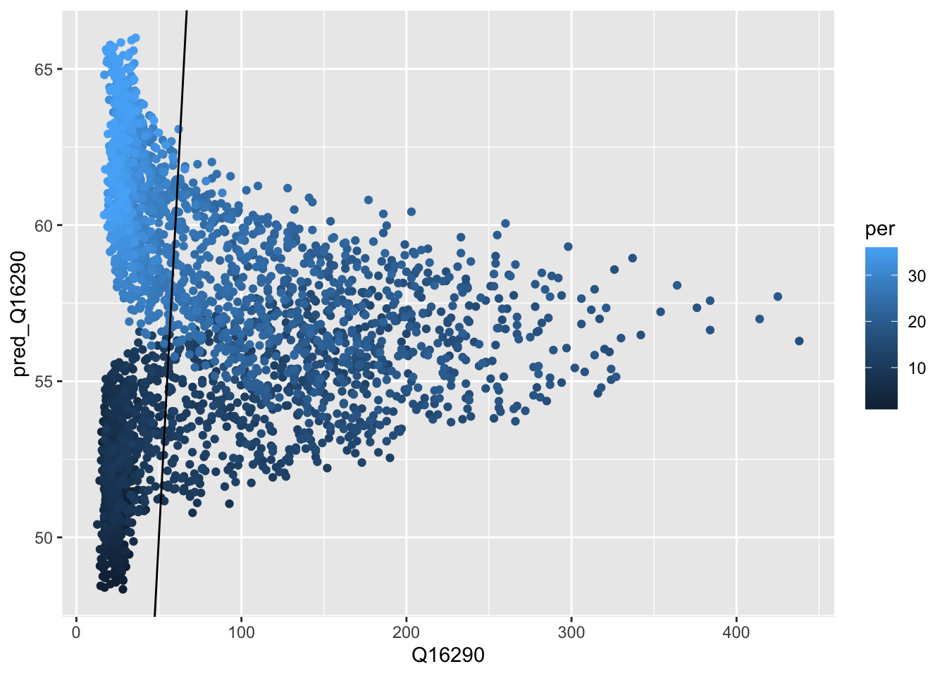
(#fig:scatterplot_Obs_vs_Fcst)Scatterplot of observed versus calculated values.
We do not seem to make a systematic error as also confirmed by inspecting the histogram or errors (they are nicely centered around 0).
ggplot(obs_pred_wide_tbl,aes(x=error)) +
  geom_histogram(bins=100)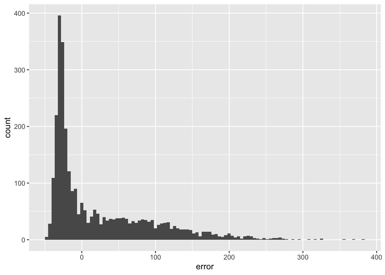
In Section @ref(Chap9_Autocorrelations) above, we saw that the PAC function is very high at lag 1. We exploit this fact be incorporating in the regression equation the observed previous discharge, i.e. \(y_{t-1}\) at time \(t-1\) to predict discharge at time \(t\). Hence, our regression can be written as
\[ y_{t} = \beta_{0} + \beta_{1} t + \beta_{2} y_{t-1} + \sum_{j=2}^{36} \beta_{j} \delta_{t}^{j} + \epsilon_{t} \]
where the \(\delta_t^{j}\) correspondingly are the 35 indicator variables as discussed above in the case of quarterly time series where we had 3 of these variables included. Before we can estimate this model, we prepare a tibble with the relevant data as shown in the table below (note that we simply renamed the discharge column to Q out of convenience).
model_data <- data_wide_tbl %>%
  dplyr::select(date,Q16290,per) %>%
  rename(Q=Q16290) %>%
  mutate(Q = log1p(Q)) %>%
  mutate(Q_lag1 = lag(Q,1))
model_data
## # A tibble: 2,985 x 4
## date Q per Q_lag1
## <date> <dbl> <int> <dbl>
## 1 1933-01-10 3.37 1 NA
## 2 1933-01-20 3.23 2 3.37
## 3 1933-01-31 3.17 3 3.23
## 4 1933-02-10 3.21 4 3.17
## 5 1933-02-20 3.26 5 3.21
## 6 1933-02-28 3.28 6 3.26
## 7 1933-03-10 3.30 7 3.28
## 8 1933-03-20 3.53 8 3.30
## 9 1933-03-31 3.57 9 3.53
## 10 1933-04-10 3.92 10 3.57
## # … with 2,975 more rowsNotice that to accommodate the \(y_{t-1}\) in the data, we simply add a column that contains a lagged version of the discharge time series itself (see column Q_lag1). Now, for example, for our regression we have a first complete set of data points on \(t = '1933-01-20'\), with \(Q=3.226844\), \(dec=2\) and \(Q_{lag1}=3.374169\). Notice how the last value corresponds to the previously observed and now known \(y_{t-1}\).
# Specification of the model formula
model_formula <- as.formula(Q ~ as.numeric(date) + per + Q_lag1)
# Note that we use na.omit() to delete incomplete data records, ie. the first observation where we lack the lagged value of the discharge.
model_data %>%  na.omit() %>% lm(formula = model_formula) %>% summary()
##
## Call:
## lm(formula = model_formula, data = .)
##
## Residuals:
## Min 1Q Median 3Q Max
## -1.09294 -0.12965 -0.03140 0.07656 1.17980
##
## Coefficients:
## Estimate Std. Error t value Pr(>|t|)
## (Intercept) 1.955e-01 1.801e-02 10.850 <2e-16 ***
## as.numeric(date) -6.402e-08 3.925e-07 -0.163 0.87
## per -7.010e-03 3.355e-04 -20.897 <2e-16 ***
## Q_lag1 9.838e-01 4.353e-03 225.992 <2e-16 ***
## ---
## Signif. codes: 0 '***' 0.001 '**' 0.01 '*' 0.05 '.' 0.1 ' ' 1
##
## Residual standard error: 0.1873 on 2980 degrees of freedom
## Multiple R-squared: 0.9453, Adjusted R-squared: 0.9452
## F-statistic: 1.716e+04 on 3 and 2980 DF, p-value: < 2.2e-16It looks like we have made a decisive step in the right direction by incorporating the previously observed discharge value. Also, notice that some of the decade factors have lost their statistical significance meaning that the seasonality can now be captured in part also by the lagged version of the time series.
Let us visualize the results quickly (tip: also zoom in to explore the fit).
model_data %>%
  na.omit() %>%
  plot_time_series_regression(
  .date_var         = date,
  .formula          = model_formula,
  .show_summary     = FALSE, # We do show the summary since we have plotted the summary output already above.
  .title            = ""
)
(#fig:lag_trend_season_Model)Linear regression model results with trend, seasonality and lag 1 predictors.
This is clearly an astonishing result. Nevertheless, we should keep a couple of things in mind:
- What about the rate of change of the discharge and the acceleration of discharge? Would the incorporation of these features help to improve the model?
- We have not assess the quality of the forecasts using the stringent quality criteria as they exist in the Central Asian Hydrometeorological Services. How does our forecast perform under this criteria?
- Does the incorporation of precipitation and temperature data help to improve our forecast skills?
- We did not test our model on out-of-sample data. Maybe our model does not generalize well? We will discuss these and related issues soon when using more advanced models but for the time being declare this a benchmark model due to its simplicity and predictive power.
We will work on these questions now and focus first on the incorporation of the rate of change in discharge and the acceleration of discharge over time. First, we add \(Q_{lag2}\) to our model data and then compute change and acceleration accordingly.
model_data <- model_data %>%
  mutate(Q_lag2 = lag(Q,2)) %>%
  mutate(change = Q_lag1 -Q_lag2) %>% # that is the speed of change in discharge
  mutate(change_lag1 = lag(change,1)) %>%
  mutate(acc = change - change_lag1) %>% na.omit() # and that is the acceleration of discharge
model_data
## # A tibble: 2,982 x 8
## date Q per Q_lag1 Q_lag2 change change_lag1 acc
## <date> <dbl> <int> <dbl> <dbl> <dbl> <dbl> <dbl>
## 1 1933-02-10 3.21 4 3.17 3.23 -0.0614 -0.147 0.0860
## 2 1933-02-20 3.26 5 3.21 3.17 0.0413 -0.0614 0.103
## 3 1933-02-28 3.28 6 3.26 3.21 0.0551 0.0413 0.0138
## 4 1933-03-10 3.30 7 3.28 3.26 0.0152 0.0551 -0.0399
## 5 1933-03-20 3.53 8 3.30 3.28 0.0187 0.0152 0.00348
## 6 1933-03-31 3.57 9 3.53 3.30 0.231 0.0187 0.212
## 7 1933-04-10 3.92 10 3.57 3.53 0.0432 0.231 -0.187
## 8 1933-04-20 4.05 11 3.92 3.57 0.348 0.0432 0.305
## 9 1933-04-30 4.47 12 4.05 3.92 0.132 0.348 -0.216
## 10 1933-05-10 4.88 13 4.47 4.05 0.416 0.132 0.284
## # … with 2,972 more rows# Specification of the model formula
model_formula <- as.formula(Q ~ as.numeric(date) + per + Q_lag1 + change + acc)
model_data %>% na.omit() %>%
plot_time_series_regression(
.date_var = date,
.formula = model_formula,
.show_summary = TRUE, # We do show the summary since we have plotted the summary output already above.
.title = ""
)##
## Call:
## stats::lm(formula = .formula, data = .data)
##
## Residuals:
## Min 1Q Median 3Q Max
## -1.01892 -0.09223 -0.02294 0.05501 1.16531
##
## Coefficients:
## Estimate Std. Error t value Pr(>|t|)
## (Intercept) 2.574e-01 1.626e-02 15.830 <2e-16 ***
## as.numeric(date) -1.834e-07 3.480e-07 -0.527 0.598
## per -2.859e-03 3.318e-04 -8.616 <2e-16 ***
## Q_lag1 9.496e-01 4.087e-03 232.331 <2e-16 ***
## change 5.650e-01 2.002e-02 28.221 <2e-16 ***
## acc -2.215e-01 1.806e-02 -12.265 <2e-16 ***
## ---
## Signif. codes: 0 '***' 0.001 '**' 0.01 '*' 0.05 '.' 0.1 ' ' 1
##
## Residual standard error: 0.1658 on 2976 degrees of freedom
## Multiple R-squared: 0.9571, Adjusted R-squared: 0.957
## F-statistic: 1.328e+04 on 5 and 2976 DF, p-value: < 2.2e-16model <- model_data %>% lm(formula=model_formula)
model %>% summary()##
## Call:
## lm(formula = model_formula, data = .)
##
## Residuals:
## Min 1Q Median 3Q Max
## -1.01892 -0.09223 -0.02294 0.05501 1.16531
##
## Coefficients:
## Estimate Std. Error t value Pr(>|t|)
## (Intercept) 2.574e-01 1.626e-02 15.830 <2e-16 ***
## as.numeric(date) -1.834e-07 3.480e-07 -0.527 0.598
## per -2.859e-03 3.318e-04 -8.616 <2e-16 ***
## Q_lag1 9.496e-01 4.087e-03 232.331 <2e-16 ***
## change 5.650e-01 2.002e-02 28.221 <2e-16 ***
## acc -2.215e-01 1.806e-02 -12.265 <2e-16 ***
## ---
## Signif. codes: 0 '***' 0.001 '**' 0.01 '*' 0.05 '.' 0.1 ' ' 1
##
## Residual standard error: 0.1658 on 2976 degrees of freedom
## Multiple R-squared: 0.9571, Adjusted R-squared: 0.957
## F-statistic: 1.328e+04 on 5 and 2976 DF, p-value: < 2.2e-16# Here, we add the the prediction to our tibble so that we can assess model predictive quality later.
model_fc_wide_tbl <- model_data %>%
mutate(pred = predict(model)) %>%
mutate(obs = expm1(Q), pred = expm1(pred)) %>%
dplyr::select(date,obs,pred,per)
model_fc_wide_tbl## # A tibble: 2,982 x 4
## date obs pred per
## <date> <dbl> <dbl> <int>
## 1 1933-02-10 23.7 23.6 4
## 2 1933-02-20 25.1 25.9 5
## 3 1933-02-28 25.5 28.0 6
## 4 1933-03-10 26 28.1 7
## 5 1933-03-20 33 28.3 8
## 6 1933-03-31 34.5 38.1 9
## 7 1933-04-10 49.3 38.9 10
## 8 1933-04-20 56.4 58.0 11
## 9 1933-04-30 86 65.3 12
## 10 1933-05-10 130 102. 13
## # … with 2,972 more rowsAnother, albeit small improvement in the forecast of predicting discharge 1-step ahead! It is now time to properly gauge the quality of this seemingly excellent model. Does it conform to local quality standards that apply to decadal forecasts? The Figure @ref(benchmarkModel_obs_pred_comparison) shows the un-transformed data. We see that we are not doing so well during the summer peak flows. As we shall see further below, these are the notoriously hard to predict values, even just for 1-step ahead decadal predictions.
model_fc_wide_tbl %>%
  dplyr::select(-per) %>%
  pivot_longer(-date) %>%
  plot_time_series(date,
                   value,
                   name,
                   .smooth = F,
                   .title = "")
7.5.3 Assessing the Quality of Forecasts
How well are we doing with our simple linear model? Let us assess the model quality using the local practices. For the Central Asian Hydromets, a forecast at a particular decade \(d\) is considered to be excellent if the following holds true
\[ |Q_{obs}(d,y) - Q_{pred}(d,y)| \le 0.674 \cdot \sigma[\Delta Q(d)] \] where \(Q_{obs}(d,y)\) is the observed discharge at decade \(d\) and year \(d\), \(Q_{pred}(d,y)\) is the predicted discharge at decade \(d\) and year \(y\), \(|Q_{obs}(d) - Q_{pred}(d)|\) thus the absolute error and \(\sigma[\Delta Q(d)] = \sigma[Q(d) - Q(d-1)]\) is the standard deviation of the difference of decadal observations at decade \(d\) and \(d-1\) over the entire observation record (hence, the year indicator \(y\) is omitted there). The equation above can be reformulated to
\[ \frac{|Q_{obs}(d,y) - Q_{pred}(d,y)|}{\sigma[\Delta Q(d)]} \le 0.674 \] So let us assess the forecast performance over the entire record using the `riversCentralAsia::assess_fc_qual`` function. Note that the function returns a list of three objects. First, it returns a tibble of the number of forecasts that are of acceptable quality for the corresponding period (i.e. decade or month) as a percentage of the total number of observations that are available for that particular period. Second, it returns the period-averaged mean and third a figure that shows forecast quality in two panels.
So, for our model which we consiedered to be performing well above, we get the following performance specs
plot01 <- TRUE
te <- assess_fc_qual(model_fc_wide_tbl,plot01)
## Registered S3 method overwritten by 'GGally':
## method from
## +.gg ggplot2te[[3]]
In other words, roughly two thirds of our in-sample forecasts comply will be considered good enough when measured according to the quality criterion. Furthermore, the model performs worse than average during the second quarter (Q2) decades, i.e. from decade 10 through 17. This is an indication that providing good forecasts in Q2 might be hard.
It is, however, generally not considered to be good practice to assess model quality on in-sample data. Rather, model performance should be assessed on out-of-sample data that was not used for model training and is thus data that is entirely unseen.
7.5.4 Generating and Assessing Out-of-Sample Forecasts
We start off with our model_data tibble and want to divide it into two sets, one for model training and one for model testing. We refer to these sets as training set and test set. For the creation of these sets, we can use the timetk::time_series_split() function.